Here comes the SU(N): multivariate quantum gates and gradients

Author: David Wierichs — Posted: 03 April 2023.

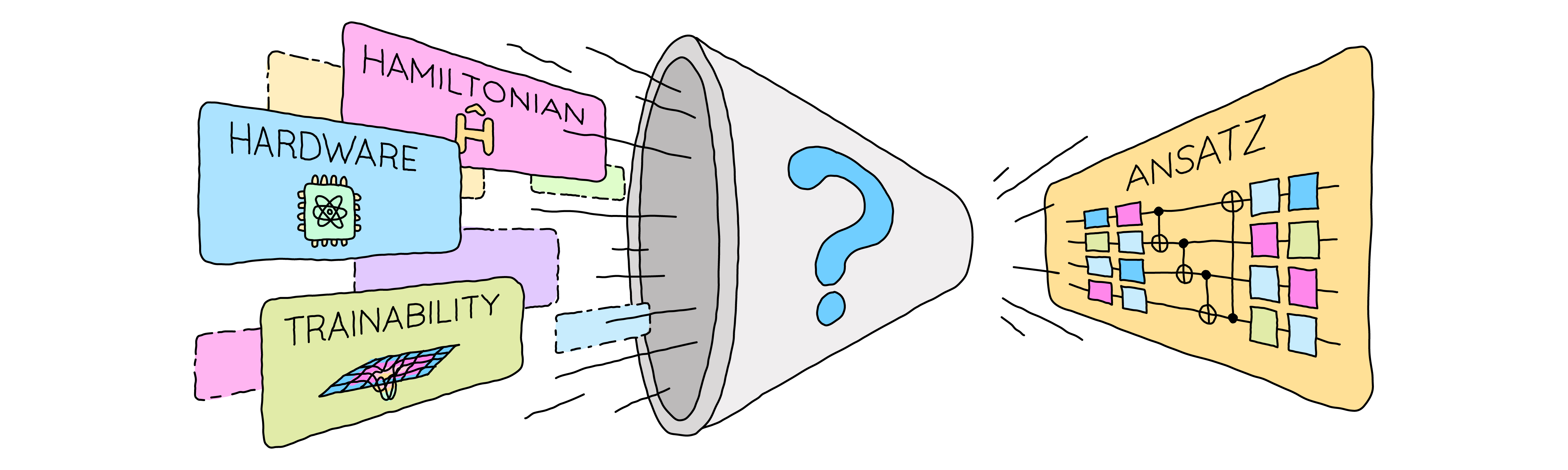
How do we choose an ansatz when designing a quantum circuit for a variational quantum algorithm? And what happens if we do not start with elementary hardware-friendly gates and compose them, but we instead use a more complex building block for local qubit interactions and allow for multi-parameter gates from the start? Can we differentiate such circuits, and how do they perform in optimization tasks?

Let’s find out!

In this tutorial, you will learn about the \(\mathrm{SU}(N)\) gate SpecialUnitary, a particular quantum gate which can act like any gate on its qubits by choosing the parameters accordingly. We will look at a custom derivative rule 2 for this gate and compare it to two alternative differentiation strategies, namely finite differences and the stochastic parameter-shift rule. Finally, we will compare the performance of qml.SpecialUnitary for a toy minimization problem to that of two other general local gates. That is, we compare the trainability of equally expressive ansätze.

Ansätze, so many ansätze

Variational quantum algorithms have been promoted to be useful for many applications. When designing these algorithms, a central task is to choose the quantum circuit ansatz, which provides a parameterization of quantum states. In the course of a variational algorithm, the circuit parameters are then optimized in order to minimize some cost function. The choice of the ansatz can have a big impact on the quantum states that can be found by the algorithm (expressivity) and on the optimization’s behaviour (trainability).

Typically, it also affects the computational cost of executing the algorithm on quantum hardware and the strength of the noise that enters the computation. Finally, the application itself influences, or even fixes, the choice of ansatz for some variational quantum algorithms, which can lead to constraints in the ansatz design.

While a number of best practices for ansatz design have been developed, a lot is still unknown about the connection between circuit structures and the resulting properties. Therefore, circuit design is often also based on intuition or heuristics; an ansatz reported in the literature might just have turned out to work particularly well for a given problem or might fall into a “standard” category of circuits.

If the application does not constrain the choice of ansatz, we may want to avoid choosing somewhat arbitrary circuit ansätze that may introduce undesirable biases. Instead, we will want to reflect the generic structure of the problem by performing a fully general operation on the qubit register. However, if we were to do so, the number of parameters required to produce such a general operation would grow much too quickly. Instead, we want to consider fully general operations on a few qubits and compose them into a fabric of local gates. For two-qubit operations, the fabric could look like this:

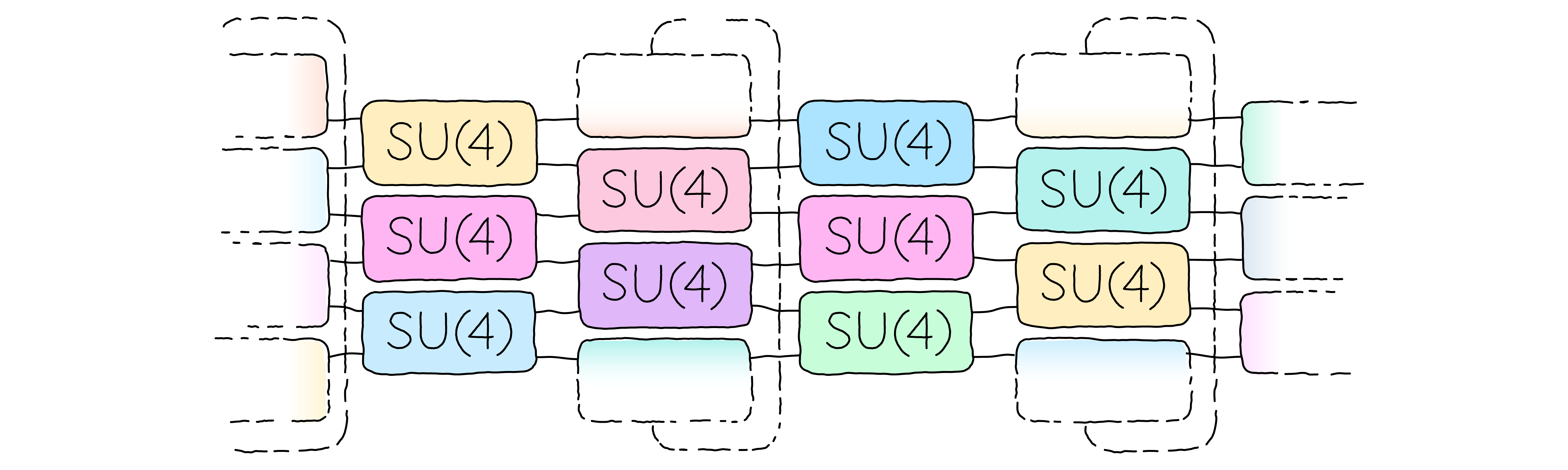
The general local operation can be implemented by composing a suitable combination of elementary gates, like single-qubit rotations and CNOT gates. Alternatively, we may choose a canonical parameterization of the group that contains all local operations, and we will see that this is an advantageous approach for the trainability of the ansatz.

Before we can use the \(\mathrm{SU}(N)\) gate in training, we will need to learn how to differentiate it in a quantum circuit. But first things first: let’s start with a brief math intro — no really, just a Liettle bit.

The special unitary group SU(N) and its Lie algebra

The gate we will look at is given by a specific parameterization of the special unitary group \(\mathrm{SU}(N)\), where \(N=2^n\) is the Hilbert space dimension of the gate for \(n\) qubits. Mathematically, the group can be defined as the set of operators (or matrices) that can be inverted by taking their adjoint and that have determinant \(1\). In general, all quantum gates acting on \(n\) qubits are elements of \(\mathrm{SU}(N)\) up to a global phase.

The group \(\mathrm{SU}(N)\) is a Lie group, and its associated Lie algebra is \(\mathfrak{su}(N)\). For our purposes, it will be sufficient to look at a matrix representation of the algebra and we may define it as

\[\mathfrak{su}(N) = \{\Omega \in \mathbb{C}^{N\times N}: \Omega^\dagger=-\Omega, \operatorname{Tr}[\Omega]=0\}.\]

The conditions are that the elements \(\Omega\) are skew-Hermitian and that their trace vanishes. We will use so-called canonical coordinates for the algebra which are simply the coefficients in the Pauli basis. That is, we consider the Pauli basis elements multiplied with the imaginary unit \(i\), except for the identity:

\[G_m \in \mathcal{P}^{(n)} = i \left\{I,X,Y,Z\right\}^n \setminus \{i I^n\}.\]

A Lie algebra element \(\Omega\) can be written as

\[\Omega = \sum_{m=1}^d \theta_m G_m,\quad \theta_m \in \mathbb{R}\]

and those coefficients \(\theta\) are precisely the canonical coordinates. You may ask why we included the prefactor \(i\) in the definition of \(G_m\) and why we excluded the identity (times \(i\)). This was done to match the properties of \(\mathfrak{su}(N)\); the prefactor makes the basis elements skew-Hermitian and the identity would not have a vanishing trace. Indeed, one can check that the dimension of \(\mathfrak{su}(N)\) is \(4^n-1\) and that there are \(4^n\) Pauli words, so that one Pauli word — the identity — had to go in any case… We can use the canonical coordinates of the algebra to express a group element in \(\mathrm{SU}(N)\) as well, and the qml.SpecialUnitary gate we will use is defined as

\[U(\boldsymbol{\theta}) = \exp\left\{\sum_{m=1}^d \theta_m G_m \right\}.\]

The number of coordinates and Pauli words in \(\mathcal{P}^{(n)}\) is \(d=4^n-1\). Therefore, this will be the number of parameters that a single qml.SpecialUnitary gate acting on \(n\) qubits will take. For example, it takes just three parameters for a single qubit, which is why Rot and U3 take three parameters and may produce any single-qubit rotation. It takes a modest 15 parameters for two qubits, but it already requires 63 parameters for three qubits.

For unitaries generated by a single operator, i.e. of the form \(\exp(i\theta G)\), there is a plethora of differentiation techniques that allow us to compute its derivative. However, a standard parameter-shift rule, for example, will not do the job if there are non-commuting terms \(G_m\) in the multi-parameter gate \(U(\boldsymbol{\theta})\) above. So how do we compute the derivative?

Obtaining the gradient

In variational quantum algorithms, we typically use the circuit to prepare a quantum state and then we measure some observable \(H\). The resulting real-valued output is considered to be the cost function \(C\) that should be minimized. If we want to use gradient-based optimization for this task, we need a method to compute the gradient \(\nabla C\) in addition to the cost function itself. As derived in the publication 2, this is possible on quantum hardware for \(\mathrm{SU}(N)\) gates as long as the gates themselves can be implemented. The implementation in PennyLane follows the decomposition idea described in App. F3, but the main text of 2 proposes an additional method that scales better in some scenarios (the caveat being that this method requires additional gates to be available on the quantum hardware). Here, we will focus on the former method. We will not go through the entire derivation, but note the following key points:

• The gradient with respect to all \(d\) parameters of an \(\mathrm{SU}(N)\) gate can be computed using \(2d\) auxiliary circuits. Each of the circuits contains one additional operation compared to the original circuit, namely a qml.PauliRot gate with rotation angles of \(\pm\frac{\pi}{2}\). Note that these Pauli rotations act on up to \(n\) qubits.

• This differentiation method uses automatic differentiation during compilation and classical coprocessing steps, but is compatible with quantum hardware. For large \(n\), the classical processing steps can quickly become prohibitively expensive.

• The computed gradient is not an approximative technique but allows for an exact computation of the gradient on simulators. On quantum hardware, this leads to unbiased gradient estimators.

The implementation in PennyLane takes care of creating the additional circuits and evaluating them, and with adequate post-processing we get the gradient \(\nabla C\).

Comparing gradient methods

Before we dive into using qml.SpecialUnitary in an optimization task, let’s compare a few methods to compute the gradient with respect to the parameters of such a gate. In particular, we will look at a finite difference (FD) approach, the stochastic parameter-shift rule, and the custom gradient method we described above.

For the first approach, we will use the standard central difference recipe given by

\[\partial_{\text{FD},\theta_j}C(\boldsymbol{\theta}) =\left[C\left(\boldsymbol{\theta}+\frac{\delta}{2}\boldsymbol{e}_j\right) -C\left(\boldsymbol{\theta}-\frac{\delta}{2}\boldsymbol{e}_j\right)\right] / \delta.\]

Here, \(\delta\) is a shift parameter that we need to choose and \(\boldsymbol{e}_j\) is the \(j\)-th canonical basis vector, i.e. the all-zeros vector with a one in the \(j\)-th entry. This approach is agnostic to the differentiated function and does not exploit its structure.

In contrast, the stochastic parameter-shift rule is a differentiation recipe developed particularly for multi-parameter gates like the \(\mathrm{SU}(N)\) gates 3. It involves the approximate evaluation of an integral by sampling splitting times \(\tau\) and evaluating an expression close to the non-stochastic parameter-shift rule for each sample. For more details, also consider the demo on the stochastic parameter-shift rule.

So, let’s dive into a toy example and explore the three gradient methods! We start by defining a simple one-qubit circuit that contains a single \(\mathrm{SU}(2)\) gate and measures the expectation value of \(H=\frac{3}{5} Z - \frac{4}{5} Y\). As qml.SpecialUnitary requires automatic differentiation subroutines even for the hardware-ready derivative recipe, we will make use of JAX.

import pennylane as qml
import numpy as np
import jax

jax.config.update("jax_enable_x64", True)
jax.config.update("jax_platform_name", "cpu")
jnp = jax.numpy

dev = qml.device("default.qubit", wires=1)
H = 0.6 * qml.PauliZ(0) - 0.8 * qml.PauliY(0)


def qfunc(theta):
    qml.SpecialUnitary(theta, wires=0)
    return qml.expval(H)


circuit = qml.QNode(qfunc, dev, interface="jax", diff_method="parameter-shift")

theta = jnp.array([0.4, 0.2, -0.5])

Now we need to set up the differentiation methods. For this demonstration, we will keep the first and last entry of theta fixed and only compute the gradient for the second parameter. This allows us to visualize the results easily and keeps the computational effort to a minimum.

We start with the finite-difference recipe, using a shift scale of \(\delta=0.75\). This choice of \(\delta\), which is much larger than usual for numerical differentiation on classical computers, is adapted to the scenario of shot-based gradients (see App. F2 of 2). We compute the derivative with respect to the second entry of theta, so we will use the unit vector \(e_2\):

unit_vector = np.array([0.0, 1.0, 0.0])


def central_diff_grad(theta, delta):
    plus_eval = circuit(theta + delta / 2 * unit_vector)
    minus_eval = circuit(theta - delta / 2 * unit_vector)
    return (plus_eval - minus_eval) / delta


delta = 0.75
print(f"Central difference: {central_diff_grad(theta, delta):.5f}")

Out:

Central difference: 0.42398

Next up, we implement the stochastic parameter-shift rule. Of course we do not do so in full generality, but for the particular circuit in this example. We will sample ten splitting times to obtain the gradient entry. For each splitting time, we need to insert a Pauli-\(Y\) rotation because \(\theta_2\) belongs to the Pauli-\(Y\) component of \(A(\boldsymbol{\theta})\). For this, we define an auxiliary circuit.

@jax.jit
@qml.qnode(dev, interface="jax")
def aux_circuit(theta, tau, sign):
    qml.SpecialUnitary(tau * theta, wires=0)
    # This corresponds to the parameter-shift evaluations of RY at 0
    qml.RY(-sign * np.pi / 2, wires=0)
    qml.SpecialUnitary((1 - tau) * theta, wires=0)
    return qml.expval(H)


def stochastic_parshift_grad(theta, num_samples):
    grad = 0
    splitting_times = np.random.random(size=num_samples)
    for tau in splitting_times:
        # Evaluate the two-term parameter-shift rule of the auxiliar circuit
        grad += aux_circuit(theta, tau, 1.0) - aux_circuit(theta, tau, -1.0)
    return grad / num_samples


num_samples = 10
print(f"Stochastic parameter-shift: {stochastic_parshift_grad(theta, num_samples):.5f}")

Out:

Stochastic parameter-shift: 0.51482

Finally, we can make use of the custom parameter-shift rule introduced in 2, which is readily available in PennyLane. Due to the implementation chosen internally, the full gradient is returned; we need to pick the second gradient entry manually. For this small toy problem, this is not an issue.

sun_grad = jax.grad(circuit)
print(f"Custom SU(N) gradient: {sun_grad(theta)[1]:.5f}")

Out:

Custom SU(N) gradient: 0.42609

We obtained three values for the gradient of interest, and they do not agree. So what is going on here? First, let’s use automatic differentiation to compute the exact value and see which method agrees with it (we again need to extract the corresponding entry from the full gradient).

autodiff_circuit = qml.QNode(qfunc, dev, interface="jax", diff_method="parameter-shift")
exact_grad = jax.grad(autodiff_circuit)(theta)[1]
print(f"Exact gradient: {exact_grad:.5f}")

Out:

Exact gradient: 0.42609

As we can see, automatic differentiation confirmed that the custom differentiation method gave us the correct result. Why do the other methods disagree? This is because the finite difference recipe is an approximate gradient method. This means it has an error even if all circuit evaluations are made exact (up to numerical precision) like in the example above. As for the stochastic parameter-shift rule, you may already guess why there is a deviation: indeed, the stochastic nature of this method leads to derivative values that are scattered around the true value. It is an unbiased estimator, so the average will approach the exact value with increasingly many evaluations. To demonstrate this, let’s compute the same derivative many times and plot a histogram of what we get. We’ll do so for num_samples=2, 10 and 100.

import matplotlib.pyplot as plt

plt.rcParams.update({"font.size": 12})

fig, ax = plt.subplots(1, 1, figsize=(6, 4))
colors = ["#ACE3FF", "#FF87EB", "#FFE096"]
for num_samples, color in zip([2, 10, 100], colors):
    grads = [stochastic_parshift_grad(theta, num_samples) for _ in range(1000)]
    ax.hist(grads, label=f"{num_samples} samples", alpha=0.9, color=color)
ylim = ax.get_ylim()
ax.plot([exact_grad] * 2, ylim, ls="--", c="k", label="Exact")
ax.set(xlabel=r"$\partial_{SPS,\theta_2}C(\theta)$", ylabel="Frequency", ylim=ylim)
ax.legend(loc="upper left")
plt.tight_layout()
plt.show()

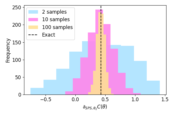
As we can see, the stochastic parameter-shift rule comes with a variance that can be reduced at the additional cost of evaluating the auxiliary circuit for more splitting times.

On quantum hardware, all measurement results are statistical in nature anyway. So how does this stochasticity combine with the three differentiation methods? We will not go into detail here, but refer to 2 to see how the custom differentiation rule proposed in the main text leads to the lowest mean squared error. For a single-qubit circuit similar to the one above, but with the single gate \(U(\boldsymbol{\theta})=\exp(iaX+ibY)\), the derivative and its expected variance are shown in the following (recoloured) plot from the manuscript:

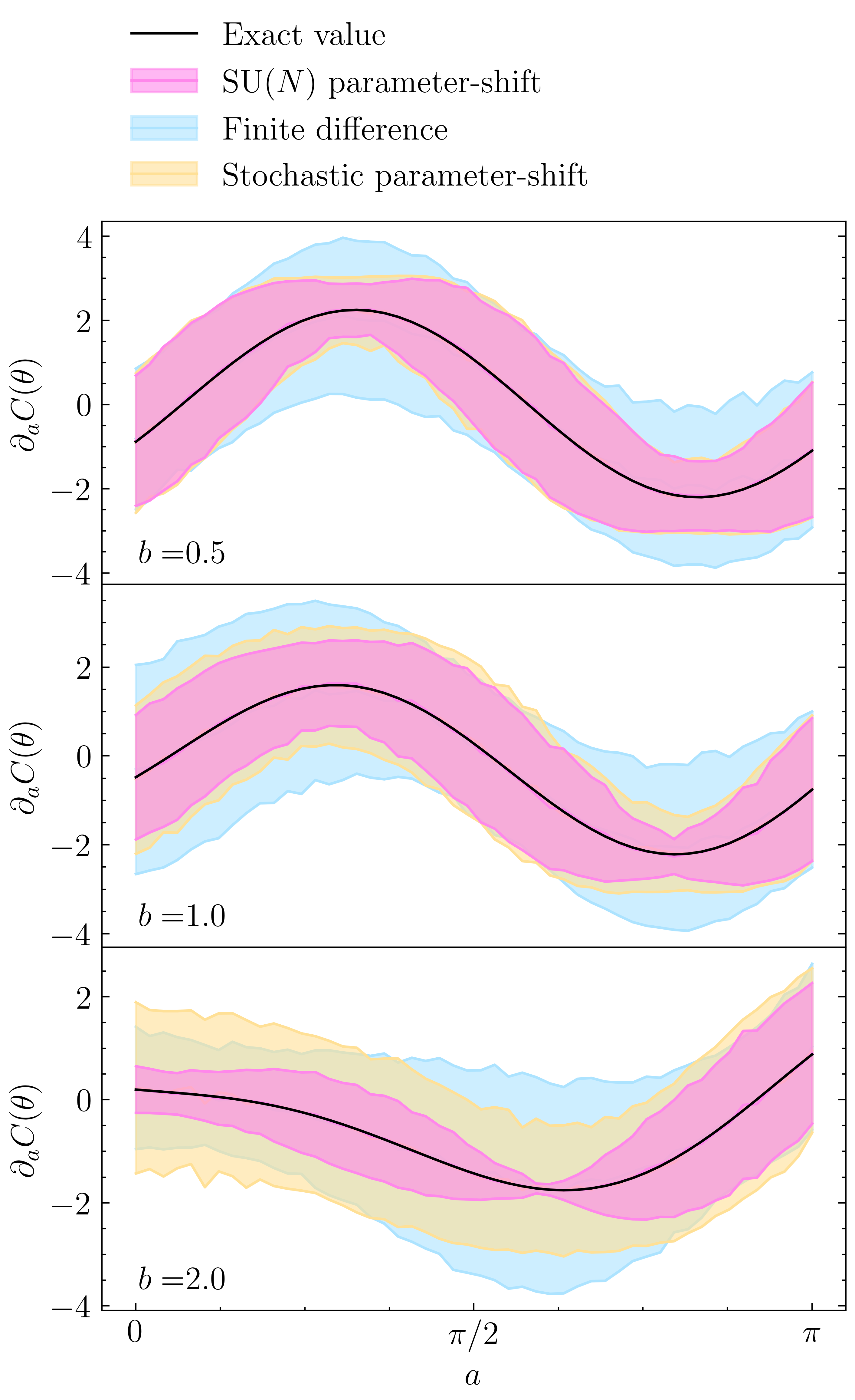
As we can see, the custom \(\mathrm{SU}(N)\) parameter-shift rule produces the gradient estimates with the smallest variance. For small values of the parameter \(b\), which is fixed for each panel, the custom shift rule and the stochastic shift rule approach the standard two-term parameter-shift rule, which would be exact for \(b=0\). The finite difference gradient shown here was obtained using the shift scale \(\delta=0.75\), as well. As we can see, this suppresses the variance down to a level comparable to those of the shift rule derivatives and this shift scale is a reasonable trade-off between the variance and the systematic error we observed earlier. As shown in App. F3 of 2, this scale is indeed close to the optimal choice if we were to compute the gradient with 100 shots per circuit.

Comparing ansatz structures

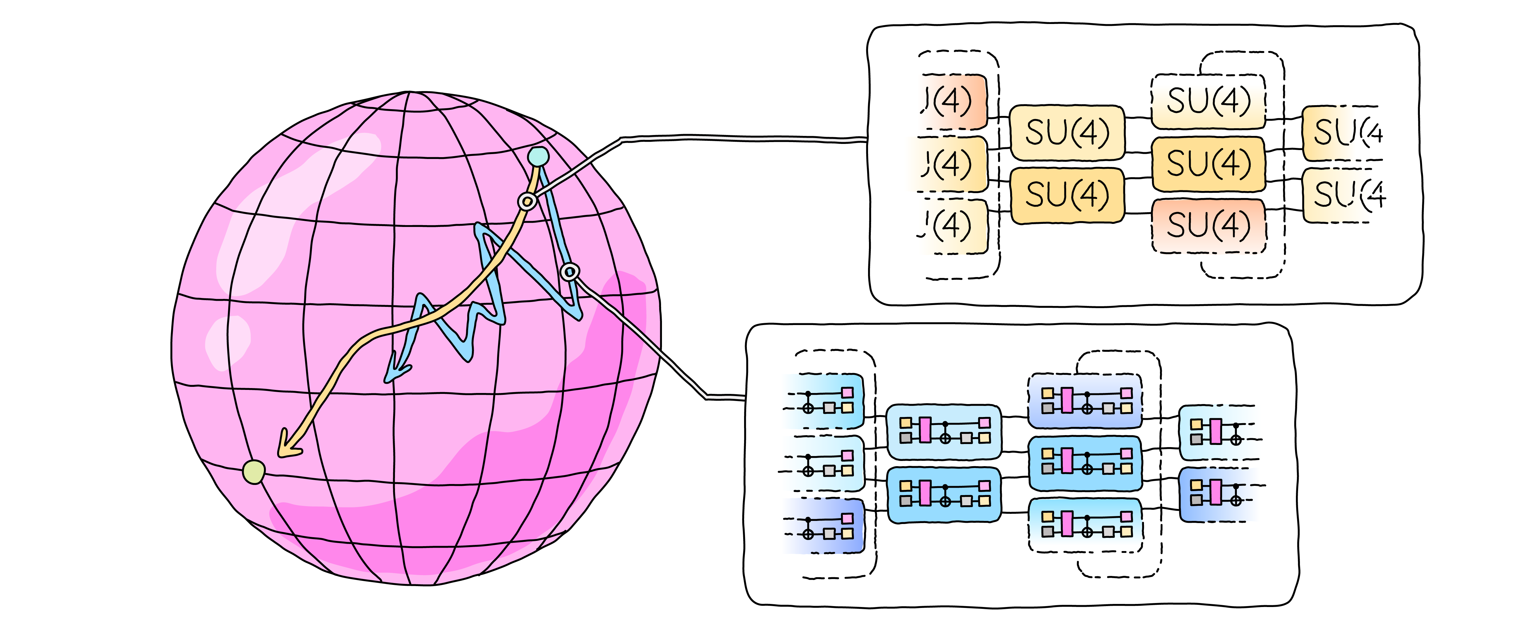
We discussed above that there are many circuit architectures available and that choosing a suitable ansatz is important but can be difficult. Here, we will compare a simple ansatz based on the qml.SpecialUnitary gate discussed above to other approaches that fully parametrize the special unitary group for the respective number of qubits. In particular, we will compare qml.SpecialUnitary to standard decompositions from the literature that parametrize \(\mathrm{SU}(N)\) with elementary gates, as well as to a sequence of Pauli rotation gates that also allows us to create any special unitary. Let us start by defining the decomposition of a two-qubit unitary. We choose the decomposition, which is optimal but not unique, from 1. The Pauli rotation sequence is available in PennyLane via qml.ArbitraryUnitary and we will not need to implement it ourselves.

def two_qubit_decomp(params, wires):
    """Implement an arbitrary SU(4) gate on two qubits
    using the decomposition from Theorem 5 in
    https://arxiv.org/pdf/quant-ph/0308006.pdf"""
    i, j = wires
    # Single U(2) parameterization on both qubits separately
    qml.Rot(*params[:3], wires=i)
    qml.Rot(*params[3:6], wires=j)
    qml.CNOT(wires=[j, i])  # First CNOT
    qml.RZ(params[6], wires=i)
    qml.RY(params[7], wires=j)
    qml.CNOT(wires=[i, j])  # Second CNOT
    qml.RY(params[8], wires=j)
    qml.CNOT(wires=[j, i])  # Third CNOT
    # Single U(2) parameterization on both qubits separately
    qml.Rot(*params[9:12], wires=i)
    qml.Rot(*params[12:15], wires=j)


# The three building blocks on two qubits we will compare are:
operations = {
    ("Decomposition", "decomposition"): two_qubit_decomp,
    ("PauliRot sequence",) * 2: qml.ArbitraryUnitary,
    ("$\mathrm{SU}(N)$ gate", "SU(N) gate"): qml.SpecialUnitary,
}

Now that we have the template for the composition approach in place, we construct a toy problem to solve using the ansätze. We will sample a random Hamiltonian in the Pauli basis (this time without the prefactor \(i\), as we want to construct a Hermitian operator) with independent coefficients that follow a normal distribution:

\[H = \sum_{m=1}^d h_m G_m,\quad h_m\sim \mathcal{N}(0,1).\]

We will work with six qubits.

num_wires = 6
wires = list(range(num_wires))
np.random.seed(62213)

coefficients = np.random.randn(4**num_wires - 1)
# Create the matrices for the entire Pauli basis
basis = qml.ops.qubit.special_unitary.pauli_basis_matrices(num_wires)
# Construct the Hamiltonian from the normal random coefficients and the basis
H_matrix = qml.math.tensordot(coefficients, basis, axes=[[0], [0]])
H = qml.Hermitian(H_matrix, wires=wires)
# Compute the ground state energy
E_min = min(qml.eigvals(H))
print(f"Ground state energy: {E_min:.5f}")

Out:

Ground state energy: -119.70320

Using the toy problem Hamiltonian and the three ansätze for \(\mathrm{SU}(N)\) operations from above, we create a circuit template that applies these operations in a brick-layer architecture with two blocks and each operation acting on loc=2 qubits. For this we define a QNode:

loc = 2
d = loc**4 - 1  # d = 15 for two-qubit operations
dev = qml.device("default.qubit", wires=num_wires)
# two blocks with two layers. Each layer contains three operations with d parameters
param_shape = (2, 2, 3, d)
init_params = np.zeros(param_shape)


def circuit(params, operation=None):
    """Apply an operation in a brickwall-like pattern to a qubit register and measure H.
    Parameters are assumed to have the dimensions (number of blocks, number of
    wires per operation, number of operations per layer, and number of parameters
    per operation), in that order.
    """
    for params_block in params:
        for i, params_layer in enumerate(params_block):
            for j, params_op in enumerate(params_layer):
                wires_op = [w % num_wires for w in range(loc * j + i, loc * (j + 1) + i)]
                operation(params_op, wires_op)
    return qml.expval(H)


qnode = qml.QNode(circuit, dev, interface="jax")
print(qml.draw(qnode)(init_params, qml.SpecialUnitary))

Out:

0: ─╭SpecialUnitary(M0)─────────────────────╭SpecialUnitary(M0)─╭SpecialUnitary(M0)
1: ─╰SpecialUnitary(M0)─╭SpecialUnitary(M0)─│───────────────────╰SpecialUnitary(M0)
2: ─╭SpecialUnitary(M0)─╰SpecialUnitary(M0)─│───────────────────╭SpecialUnitary(M0)
3: ─╰SpecialUnitary(M0)─╭SpecialUnitary(M0)─│───────────────────╰SpecialUnitary(M0)
4: ─╭SpecialUnitary(M0)─╰SpecialUnitary(M0)─│───────────────────╭SpecialUnitary(M0)
5: ─╰SpecialUnitary(M0)─────────────────────╰SpecialUnitary(M0)─╰SpecialUnitary(M0)

──────────────────────╭SpecialUnitary(M0)─┤ ╭<𝓗(M1)>
──╭SpecialUnitary(M0)─│───────────────────┤ ├<𝓗(M1)>
──╰SpecialUnitary(M0)─│───────────────────┤ ├<𝓗(M1)>
──╭SpecialUnitary(M0)─│───────────────────┤ ├<𝓗(M1)>
──╰SpecialUnitary(M0)─│───────────────────┤ ├<𝓗(M1)>
──────────────────────╰SpecialUnitary(M0)─┤ ╰<𝓗(M1)>

We can now proceed to prepare the optimization task using this circuit and an optimization routine of our choice. For simplicity, we run a vanilla gradient descent optimization with a fixed learning rate for 500 steps. Again, we use JAX

# for auto-differentiation.

learning_rate = 5e-4
num_steps = 500
init_params = jax.numpy.array(init_params)
grad_fn = jax.jit(jax.jacobian(qnode), static_argnums=1)
qnode = jax.jit(qnode, static_argnums=1)

With this configuration, let’s run the optimization!

energies = {}
for (name, print_name), operation in operations.items():
    print(f"Running the optimization for the {print_name}")
    params = init_params.copy()
    energy = []
    for step in range(num_steps):
        cost = qnode(params, operation)
        params = params - learning_rate * grad_fn(params, operation)
        energy.append(cost)  # Store energy value
        if step % 50 == 0:  # Report current energy
            print(f"{step:3d} Steps: {cost:.6f}")

    energy.append(qnode(params, operation))  # Final energy value
    energies[name] = energy

Out:

Running the optimization for the decomposition
  0 Steps: 0.108347
 50 Steps: -20.304280
100 Steps: -46.639755
150 Steps: -62.803368
200 Steps: -70.680297
250 Steps: -74.809580
300 Steps: -77.212092
350 Steps: -78.814361
400 Steps: -80.016451
450 Steps: -81.025807
Running the optimization for the PauliRot sequence
  0 Steps: 0.108347
 50 Steps: -39.877320
100 Steps: -54.140646
150 Steps: -59.806581
200 Steps: -64.677694
250 Steps: -69.808084
300 Steps: -75.313238
350 Steps: -80.848057
400 Steps: -85.016118
450 Steps: -87.853931
Running the optimization for the SU(N) gate
  0 Steps: 0.108347
 50 Steps: -63.548081
100 Steps: -84.956818
150 Steps: -94.176547
200 Steps: -100.707290
250 Steps: -104.434910
300 Steps: -106.567958
350 Steps: -108.110054
400 Steps: -109.453172
450 Steps: -110.748710

So, did it work? Judging from the intermediate energy values, it seems that the optimization outcomes differ notably. But let’s take a look at the relative error in energy across the optimization process.

fig, ax = plt.subplots(1, 1)
styles = [":", "--", "-"]
colors = ["#70CEFF", "#C756B2", "#FFE096"]
for (name, energy), c, ls in zip(energies.items(), colors, styles):
    error = (energy - E_min) / abs(E_min)
    ax.plot(list(range(len(error))), error, label=name, c=c, ls=ls, lw=2.5)

ax.set(xlabel="Iteration", ylabel="Relative error")
ax.legend()
plt.show()

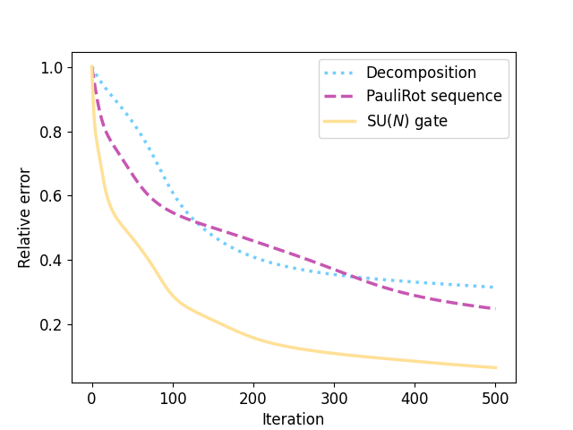
We find that the optimization indeed performs significantly better for qml.SpecialUnitary than for the other two general unitaries, while using the same number of parameters and preserving the expressibility of the circuit ansatz. This means that we found a particularly well-trainable parameterization of the local unitaries which allows us to reduce the energy of the prepared quantum state more easily while maintaining the number of parameters.

Conclusion

To summarize, in this tutorial we introduced qml.SpecialUnitary, a multi-parameter gate that can act like any gate on the qubits it is applied to and that is constructed with Lie theory in mind. We discussed three methods of differentiating quantum circuits that use this gate, showing that a new custom parameter-shift rule presented in 2 is particularly suitable to produce unbiased gradient estimates with the lowest variance. Afterwards, we used this differentiation technique when comparing the performance of qml.SpecialUnitary to that of other gates that can act like any gate locally. For this, we ran a gradient-based optimization for a toy model Hamiltonian and found that qml.SpecialUnitary is particularly well-trainable, achieving lower energies significantly quicker than the other tested gates.

There are still exciting questions to answer about qml.SpecialUnitary: How can the custom parameter-shift rule be used for other gates, and what does the so-called Dynamical Lie algebra of these gates have to do with it? How can we implement the qml.SpecialUnitary gate on hardware? Is the unitary time evolution implemented by this gate special in a physical sense?

The answers to some, but not all, of these questions can be found in 2. We are certain that there are many more interesting aspects of this gate to be uncovered! If you want to learn more, consider the other literature references below, as well as the documentation of SpecialUnitary.

References

1

Farrokh Vatan and Colin Williams, “Optimal Quantum Circuits for General Two-Qubit Gates”, arXiv:quant-ph/0308006 (2003).

2(1,2,3,4,5,6,7,8,9)

R. Wiersema, D. Lewis, D. Wierichs, J. F. Carrasquilla, and N. Killoran. “Here comes the SU(N): multivariate quantum gates and gradients” arXiv:2303.11355 (2023).

3

Leonardo Banchi and Gavin E. Crooks. “Measuring Analytic Gradients of General Quantum Evolution with the Stochastic Parameter Shift Rule.” Quantum 5, 386 (2021).

About the author

David Wierichs

David is a researcher and quantum software developer at Xanadu, who likes to think about quantum gradients and how to use them in variational quantum algorithms. He enjoys sharing ideas in science and open source software and likes implementing cool stuff in PennyLane.

demos/tutorial_here_comes_the_sun

 

Download Python script

 

Download Notebook

 

View on GitHub