Note
Click here to download the full example code
Perturbative Gadgets for Variational Quantum Algorithms
Author: Simon Cichy — Posted: 09 December 2022. Last updated: 09 December 2022.
Variational quantum algorithms are seen as one of the most primising candidates for useful applications of quantum computers in the near term, but there are still a few hurdles to overcome when it comes to practical implementation. One of them, is the trainability. In other words, one needs to ensure that the cost function is not flat. In this tutorial, we will explore the application of perturbative gadgets in variational quantum algorithms to outgo the issue of cost-function-dependent barren plateaus, as proposed in Ref. 1
Some context
Barren plateaus refer to the phenomenon where the gradients of the cost function decay exponentially with the size of the problem. Essentially, the cost landscape becomes flat, with exception of some small regions, e.g., around the minimum. That is a problem because increasing the precision of the cost function requires more measurements from the quantum device due to shot noise, and an exponential number of measurements would render the algorithm impractical. If you are not familiar yet with the concept of barren plateaus, I recommend you first check out the demonstrations on barren plateaus and avoiding barren plateaus with local cost functions.
As presented in the second aforementioned demo, barren plateaus are more severe when using global cost functions compared to local ones. A global cost function requires the simultaneous measurement of all qubits at once. In contrast, a local one is constructed from terms that only act on a small subset of qubits.
We want to explore this topic further and learn about one possible mitigation strategy. Thinking about Variational Quantum Eigensolver (VQE) applications, let us consider cost functions that are expectation values of Hamiltonians such as
Here \(|00\ldots 0\rangle\) is our initial state, \(V(\theta)\) is the circuit ansatz and \(H\) the Hamiltonian whose expectation value we need to minimize. In some cases, it is easy to find a local cost function which can substitute a global one with the same ground state. Take, for instance, the following Hamiltonians that induce global and local cost functions, respectively.
Those are two different Hamiltonians (not just different formulations of the same one), but they share the same ground state:
Therefore, one can work with either Hamiltonian to perform the VQE routine. However, it is not always so simple. What if we want to find the minimum eigenenergy of \(H = X \otimes X \otimes Y \otimes Z + Z \otimes Y \otimes X \otimes X\) ? It is not always trivial to construct a local cost function that has the same minimum as the cost function of interest. This is where perturbative gadgets come into play!
The definitions
Perturbative gadgets are a common tool in adiabatic quantum computing. Their goal is to find a Hamiltonian with local interactions that mimics another Hamiltonian with more complex couplings.
Ideally, they would want to implement the target Hamiltonian with complex couplings, but since it’s hard to implement more than few-body interactions on hardware, they cannot do so. Perturbative gadgets work by increasing the dimension of the Hilbert space (i.e., the number of qubits) and “encoding” the target Hamiltonian in the low-energy subspace of a so-called “gadget” Hamiltonian.
Let us now construct such a gadget Hamiltonian tailored for VQE applications. First, we start from a target Hamiltonian that is a linear combination of Pauli words acting on \(k\) qubits each:
where \(h_i = \sigma_{i,1} \otimes \sigma_{i,2} \otimes \ldots \otimes \sigma_{i,k}\), \(\sigma_{i,j} \in \{ X, Y, Z \}\), and \(c_i \in \mathbb{R}\). Now we construct the gadget Hamiltonian. For each term \(h_i\), we will need \(k\) additional qubits, which we call auxiliary qubits, and to add two terms to the Hamiltonian: an “unperturbed” part \(H^\text{aux}_i\) and a perturbation \(V_i\) of strength \(\lambda\). The unperturbed part penalizes each of the newly added qubits for not being in the \(|0\rangle\) state
On the other hand, the perturbation part implements one of the operators in the Pauli word \(\sigma_{i,j}\) on the corresponding qubit of the target register and a pair of Pauli \(X\) gates on two of the auxiliary qubits:
In the end,
To grasp this idea better, this is what would result from working with a Hamiltonian acting on a total of \(8\) qubits and having \(3\) terms, each of them being a \(4\)-body interaction.
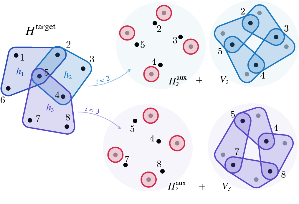
For each of the terms \(h_1\), \(h_2\), and \(h_3\) we add \(4\) auxiliary qubits. In the end, our gadget Hamiltonian acts on \(8+3\cdot 4 = 20\) qubits.
The penalization (red) acts only on the auxiliary registers, penalizing each qubit individually, while the perturbations couple the target with the auxiliary qubits.
As shown in Ref. 1, this construction results in a spectrum that, for low energies, is similar to that of the original Hamiltonian. This means that by minimizing the gadget Hamiltonian and reaching its global minimum, the resulting state will be close to the global minimum of \(H^\text{target}\).
Since it is a local cost function, it is better behaved with respect to barren plateaus than the global cost function, making it more trainable. As a result, one can mitigate the onset of cost-function-dependent barren plateaus by substituting the global cost function with the resulting gadget and using that for training instead. That is what we will do in the rest of this tutorial.
First, a few imports. PennyLane and NumPy of course, and a few
functions specific to our tutorial.
The PerturbativeGadget class allows the user to generate the gadget Hamiltonian
from a user-given target Hamiltonian in an automated way.
For those who want to check its inner workings,
you can find the code here:
barren_gadgets.py.
The functions get_parameter_shape, generate_random_gate_sequence, and
build_ansatz (for the details:
layered_ansatz.py
) are there to build the parameterized quantum circuit we use in this demo.
The first computes the shape of the array of trainable parameters that the
circuit will need. The second generates a random sequence of Pauli rotations
from \(\{R_X, R_Y, R_Z\}\) with the right dimension.
Finally, build_ansatz puts the pieces together.
import pennylane as qml
from pennylane import numpy as np
from barren_gadgets.barren_gadgets import PerturbativeGadgets
from barren_gadgets.layered_ansatz import (
    generate_random_gate_sequence,
    get_parameter_shape,
    build_ansatz,
)

np.random.seed(3)
Now, let’s take the example given above:
First, we construct our target Hamiltonian in PennyLane.
For this, we use the
Hamiltonian class.
H_target = qml.PauliX(0) @ qml.PauliX(1) @ qml.PauliY(2) @ qml.PauliZ(3) \
         + qml.PauliZ(0) @ qml.PauliY(1) @ qml.PauliX(2) @ qml.PauliX(3)
Now we can check that we constructed what we wanted.
print(H_target)
Out:
  (1) [X0 X1 Y2 Z3]
+ (1) [Z0 Y1 X2 X3]
We indeed have a Hamiltonian composed of two terms with the expected Pauli
words.
Next, we can construct the corresponding gadget Hamiltonian.
Using the class PerturbativeGadgets, we can automatically
generate the gadget Hamiltonian from the target Hamiltonian.
The object gadgetizer will contain all the information about the settings of
the gadgetization procedure (there are quite a few knobs one can tweak,
but we’ll skip that for now).
Then, the method gadgetize takes a
Hamiltonian
object and generates the
corresponding gadget Hamiltonian.
Out:
  (-0.5) [Z4]
+ (-0.5) [Z5]
+ (-0.5) [Z6]
+ (-0.5) [Z7]
+ (-0.5) [Z8]
+ (-0.5) [Z9]
+ (-0.5) [Z10]
+ (-0.5) [Z11]
+ (0.5) [I4]
+ (0.5) [I5]
+ (0.5) [I6]
+ (0.5) [I7]
+ (0.5) [I8]
+ (0.5) [I9]
+ (0.5) [I10]
+ (0.5) [I11]
+ (-0.03125) [X4 X5 X0]
+ (-0.03125) [X8 X9 Z0]
+ (0.03125) [X5 X6 X1]
+ (0.03125) [X6 X7 Y2]
+ (0.03125) [X7 X4 Z3]
+ (0.03125) [X9 X10 Y1]
+ (0.03125) [X10 X11 X2]
+ (0.03125) [X11 X8 X3]
So, let’s see what we got.
We started with 4 target qubits (labelled 0 to 3) and two 4-body terms.
Thus we get 4 additional qubits twice (4 to 11).
The first 16 elements of our Hamiltonian correspond to the unperturbed part.
The last 8 are the perturbation. They are a little scrambled, but one can
recognize the 8 Paulis from the target Hamiltonian on the qubits 0 to
3 and the cyclic pairwise \(X\) structure on the auxiliaries.
Indeed, they are \((X_4X_5, X_5X_6, X_6X_7, X_7X_4)\) and
\((X_8X_9, X_9X_{10}, X_{10}X_{11}, X_{11}X_8)\).
Training with the gadget Hamiltonian
Now that we have a little intuition on how the gadget Hamiltonian construction works, we will use it to train. Classical simulations of qubit systems are expensive, so we will simplify further to a target Hamiltonian with a single term, and show that using the gadget Hamiltonian for training allows us to minimize the target Hamiltonian. So, let us construct the two Hamiltonians of interest.
H_target = 1 * qml.PauliX(0) @ qml.PauliX(1) @ qml.PauliY(2) @ qml.PauliZ(3)
gadgetizer = PerturbativeGadgets(perturbation_factor=10)
H_gadget = gadgetizer.gadgetize(H_target)
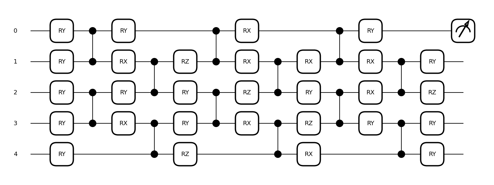
Then we need to set up our variational quantum algorithm. That is, we choose a circuit ansatz with randomly initialized weights, the cost function, the optimizer with its step size, the number of optimization steps, and the device to run the circuit on. For an ansatz, we will use a variation of the qml.SimplifiedTwoDesign, which was proposed in previous works on cost-function-dependent barren plateaus 2. I will skip the details of the construction, since it is not our focus here, and just show what it looks like. Here is the circuit for a small example
shapes = get_parameter_shape(n_layers=3, n_wires=5)
init_weights = [np.pi / 4] * shapes[0][0]
weights = np.random.uniform(0, np.pi, size=shapes[1])


@qml.qnode(qml.device("default.qubit", wires=range(5)))
def display_circuit(weights):
    build_ansatz(initial_layer_weights=init_weights, weights=weights, wires=range(5))
    return qml.expval(qml.PauliZ(wires=0))

import matplotlib.pyplot as plt
qml.draw_mpl(display_circuit)(weights)
plt.show()
Now we build the circuit for our actual experiment.
# Total number of qubits: target + auxiliary
num_qubits = 4 + 1 * 4

# Other parameters of the ansatz: weights and gate sequence
shapes = get_parameter_shape(n_layers=num_qubits, n_wires=num_qubits)
init_weights = [np.pi / 4] * shapes[0][0]
weights = np.random.uniform(0, np.pi, size=shapes[1])
random_gate_sequence = generate_random_gate_sequence(qml.math.shape(weights))
For the classical optimization, we will use the standard gradient descent algorithm and perform 500 iterations. For the quantum part, we will simulate our circuit using the default.qubit simulator.
opt = qml.GradientDescentOptimizer(stepsize=0.1)
max_iter = 500
dev = qml.device("default.qubit", wires=range(num_qubits))
Finally, we will use two cost functions and create a QNode for each. The first cost function, the training cost, is the loss function of the optimization. For the training, we use the gadget Hamiltonian. To ensure that our gadget optimization is proceeding as intended, we also define another cost function based on the target Hamiltonian. We will evaluate its value at each iteration for monitoring purposes, but it will not be used in the optimization.
@qml.qnode(dev)
def training_cost(weights):
    build_ansatz(
        initial_layer_weights=init_weights,
        weights=weights,
        wires=range(num_qubits),
        gate_sequence=random_gate_sequence,
    )
    return qml.expval(H_gadget)


@qml.qnode(dev)
def monitoring_cost(weights):
    build_ansatz(
        initial_layer_weights=init_weights,
        weights=weights,
        wires=range(num_qubits),
        gate_sequence=random_gate_sequence,
    )
    return qml.expval(H_target)
The idea is that if we reach the global minimum for the gadget Hamiltonian, we should also be close to the global minimum of the target Hamiltonian, which is what we are ultimately interested in. To see the results and plot them, we will save the cost values at each iteration.
costs_lists = {}
costs_lists["training"] = [training_cost(weights)]
costs_lists["monitoring"] = [monitoring_cost(weights)]
Now everything is set up, let’s run the optimization and see how it goes. Be careful, this will take a while.
for it in range(max_iter):
    weights = opt.step(training_cost, weights)
    costs_lists["training"].append(training_cost(weights))
    costs_lists["monitoring"].append(monitoring_cost(weights))


plt.style.use("seaborn")

plt.figure()
plt.plot(costs_lists["training"])
plt.plot(costs_lists["monitoring"])
plt.legend(["training", "monitoring"])
plt.xlabel("Number of iterations")
plt.ylabel("Cost values")
plt.show()
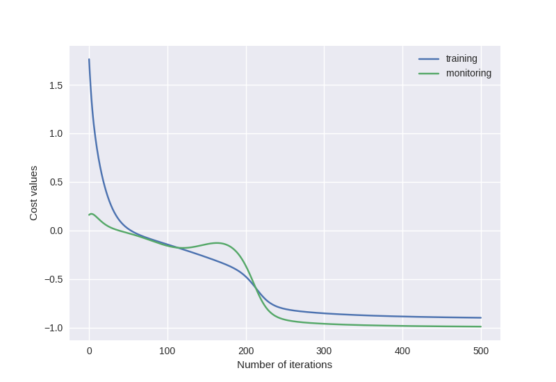
Since our example target Hamiltonian is a single Pauli string, we know without needing any training that it has only \(\pm 1\) eigenvalues. It is a very simple example, but we see that the training of our circuit using the gadget Hamiltonian as a cost function did indeed allow us to reach the global minimum of the target cost function.
Now that you have an idea of how you can use perturbative gadgets in variational quantum algorithms, you can try applying them to more complex problems! However, be aware of the exponential scaling of classical simulations of quantum systems; adding linearly many auxiliary qubits quickly becomes hard to simulate. For those interested in the theory behind it or more formal statements of “how close” the results using the gadget are from the targeted ones, check out the original paper 1. There you will also find further discussions on the advantages and limits of this proposal, as well as a more general recipe to design other gadget constructions with similar properties. Also, the complete code with explanations on how to reproduce the figures from the paper can be found in this repository.
References
- 1(1,2,3)
Cichy, S., Faehrmann, P.K., Khatri, S., Eisert, J. “A perturbative gadget for delaying the onset of barren plateaus in variational quantum algorithms.” arXiv:2210.03099, 2022.
- 2
Cerezo, M., Sone, A., Volkoff, T. et al. “Cost function dependent barren plateaus in shallow parametrized quantum circuits.” Nat Commun 12, 1791, 2021.