QAOA for MaxCut

Author: Angus Lowe — Posted: 11 October 2019. Last updated: 13 April 2021.

In this tutorial we implement the quantum approximate optimization algorithm (QAOA) for the MaxCut problem as proposed by Farhi, Goldstone, and Gutmann (2014). First, we give an overview of the MaxCut problem using a simple example, a graph with 4 vertices and 4 edges. We then show how to find the maximum cut by running the QAOA algorithm using PennyLane.

Background

The MaxCut problem

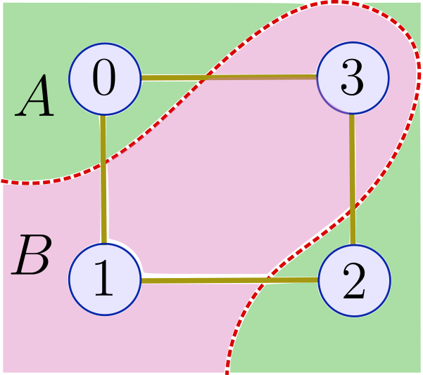
The aim of MaxCut is to maximize the number of edges (yellow lines) in a graph that are “cut” by a given partition of the vertices (blue circles) into two sets (see figure below).

Consider a graph with \(m\) edges and \(n\) vertices. We seek the partition \(z\) of the vertices into two sets \(A\) and \(B\) which maximizes

\[C(z) = \sum_{\alpha=1}^{m}C_\alpha(z),\]

where \(C\) counts the number of edges cut. \(C_\alpha(z)=1\) if \(z\) places one vertex from the \(\alpha^\text{th}\) edge in set \(A\) and the other in set \(B\), and \(C_\alpha(z)=0\) otherwise. Finding a cut which yields the maximum possible value of \(C\) is an NP-complete problem, so our best hope for a polynomial-time algorithm lies in an approximate optimization. In the case of MaxCut, this means finding a partition \(z\) which yields a value for \(C(z)\) that is close to the maximum possible value.

We can represent the assignment of vertices to set \(A\) or \(B\) using a bitstring, \(z=z_1...z_n\) where \(z_i=0\) if the \(i^\text{th}\) vertex is in \(A\) and \(z_i = 1\) if it is in \(B\). For instance, in the situation depicted in the figure above the bitstring representation is \(z=0101\text{,}\) indicating that the \(0^{\text{th}}\) and \(2^{\text{nd}}\) vertices are in \(A\) while the \(1^{\text{st}}\) and \(3^{\text{rd}}\) are in \(B\). This assignment yields a value for the objective function (the number of yellow lines cut) \(C=4\), which turns out to be the maximum cut. In the following sections, we will represent partitions using computational basis states and use PennyLane to rediscover this maximum cut.

Note

In the graph above, \(z=1010\) could equally well serve as the maximum cut.

A circuit for QAOA

This section describes implementing a circuit for QAOA using basic unitary gates to find approximate solutions to the MaxCut problem. Firstly, denoting the partitions using computational basis states \(|z\rangle\), we can represent the terms in the objective function as operators acting on these states

\[C_\alpha = \frac{1}{2}\left(1-\sigma_{z}^j\sigma_{z}^k\right),\]

where the \(\alpha\text{th}\) edge is between vertices \((j,k)\). \(C_\alpha\) has eigenvalue 1 if and only if the \(j\text{th}\) and \(k\text{th}\) qubits have different z-axis measurement values, representing separate partitions. The objective function \(C\) can be considered a diagonal operator with integer eigenvalues.

QAOA starts with a uniform superposition over the \(n\) bitstring basis states,

\[|+_{n}\rangle = \frac{1}{\sqrt{2^n}}\sum_{z\in \{0,1\}^n} |z\rangle.\]

We aim to explore the space of bitstring states for a superposition which is likely to yield a large value for the \(C\) operator upon performing a measurement in the computational basis. Using the \(2p\) angle parameters \(\boldsymbol{\gamma} = \gamma_1\gamma_2...\gamma_p\), \(\boldsymbol{\beta} = \beta_1\beta_2...\beta_p\) we perform a sequence of operations on our initial state:

\[|\boldsymbol{\gamma},\boldsymbol{\beta}\rangle = U_{B_p}U_{C_p}U_{B_{p-1}}U_{C_{p-1}}...U_{B_1}U_{C_1}|+_n\rangle\]

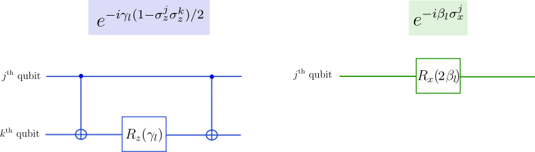
where the operators have the explicit forms

\[\begin{split}U_{B_l} &= e^{-i\beta_lB} = \prod_{j=1}^n e^{-i\beta_l\sigma_x^j}, \\ U_{C_l} &= e^{-i\gamma_lC} = \prod_{\text{edge (j,k)}} e^{-i\gamma_l(1-\sigma_z^j\sigma_z^k)/2}.\end{split}\]

In other words, we make \(p\) layers of parametrized \(U_bU_C\) gates. These can be implemented on a quantum circuit using the gates depicted below, up to an irrelevant constant that gets absorbed into the parameters.

Let \(\langle \boldsymbol{\gamma}, \boldsymbol{\beta} | C | \boldsymbol{\gamma},\boldsymbol{\beta} \rangle\) be the expectation of the objective operator. In the next section, we will use PennyLane to perform classical optimization over the circuit parameters \((\boldsymbol{\gamma}, \boldsymbol{\beta})\). This will specify a state \(|\boldsymbol{\gamma},\boldsymbol{\beta}\rangle\) which is likely to yield an approximately optimal partition \(|z\rangle\) upon performing a measurement in the computational basis. In the case of the graph shown above, we want to measure either 0101 or 1010 from our state since these correspond to the optimal partitions.

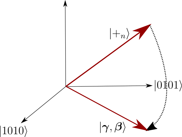
Qualitatively, QAOA tries to evolve the initial state into the plane of the \(|0101\rangle\), \(|1010\rangle\) basis states (see figure above).

Implementing QAOA in PennyLane

Imports and setup

To get started, we import PennyLane along with the PennyLane-provided version of NumPy.

import pennylane as qml
from pennylane import numpy as np

np.random.seed(42)

Operators

We specify the number of qubits (vertices) with n_wires and compose the unitary operators using the definitions above. \(U_B\) operators act on individual wires, while \(U_C\) operators act on wires whose corresponding vertices are joined by an edge in the graph. We also define the graph using the list graph, which contains the tuples of vertices defining each edge in the graph.

n_wires = 4
graph = [(0, 1), (0, 3), (1, 2), (2, 3)]

# unitary operator U_B with parameter beta
def U_B(beta):
    for wire in range(n_wires):
        qml.RX(2 * beta, wires=wire)


# unitary operator U_C with parameter gamma
def U_C(gamma):
    for edge in graph:
        wire1 = edge[0]
        wire2 = edge[1]
        qml.CNOT(wires=[wire1, wire2])
        qml.RZ(gamma, wires=wire2)
        qml.CNOT(wires=[wire1, wire2])

We will need a way to convert a bitstring, representing a sample of multiple qubits in the computational basis, to integer or base-10 form.

def bitstring_to_int(bit_string_sample):
    bit_string = "".join(str(bs) for bs in bit_string_sample)
    return int(bit_string, base=2)

Circuit

Next, we create a quantum device with 4 qubits.

dev = qml.device("default.qubit", wires=n_wires, shots=1)

We also require a quantum node which will apply the operators according to the angle parameters, and return the expectation value of the observable \(\sigma_z^{j}\sigma_z^{k}\) to be used in each term of the objective function later on. The argument edge specifies the chosen edge term in the objective function, \((j,k)\). Once optimized, the same quantum node can be used for sampling an approximately optimal bitstring if executed with the edge keyword set to None. Additionally, we specify the number of layers (repeated applications of \(U_BU_C\)) using the keyword n_layers.

@qml.qnode(dev)
def circuit(gammas, betas, edge=None, n_layers=1):
    # apply Hadamards to get the n qubit |+> state
    for wire in range(n_wires):
        qml.Hadamard(wires=wire)
    # p instances of unitary operators
    for i in range(n_layers):
        U_C(gammas[i])
        U_B(betas[i])
    if edge is None:
        # measurement phase
        return qml.sample()
    # during the optimization phase we are evaluating a term
    # in the objective using expval
    H = qml.PauliZ(edge[0]) @ qml.PauliZ(edge[1])
    return qml.expval(H)

Optimization

Finally, we optimize the objective over the angle parameters \(\boldsymbol{\gamma}\) (params[0]) and \(\boldsymbol{\beta}\) (params[1]) and then sample the optimized circuit multiple times to yield a distribution of bitstrings. One of the optimal partitions (\(z=0101\) or \(z=1010\)) should be the most frequently sampled bitstring. We perform a maximization of \(C\) by minimizing \(-C\), following the convention that optimizations are cast as minimizations in PennyLane.

def qaoa_maxcut(n_layers=1):
    print("\np={:d}".format(n_layers))

    # initialize the parameters near zero
    init_params = 0.01 * np.random.rand(2, n_layers, requires_grad=True)

    # minimize the negative of the objective function
    def objective(params):
        gammas = params[0]
        betas = params[1]
        neg_obj = 0
        for edge in graph:
            # objective for the MaxCut problem
            neg_obj -= 0.5 * (1 - circuit(gammas, betas, edge=edge, n_layers=n_layers))
        return neg_obj

    # initialize optimizer: Adagrad works well empirically
    opt = qml.AdagradOptimizer(stepsize=0.5)

    # optimize parameters in objective
    params = init_params
    steps = 30
    for i in range(steps):
        params = opt.step(objective, params)
        if (i + 1) % 5 == 0:
            print("Objective after step {:5d}: {: .7f}".format(i + 1, -objective(params)))

    # sample measured bitstrings 100 times
    bit_strings = []
    n_samples = 100
    for i in range(0, n_samples):
        bit_strings.append(bitstring_to_int(circuit(params[0], params[1], edge=None, n_layers=n_layers)))

    # print optimal parameters and most frequently sampled bitstring
    counts = np.bincount(np.array(bit_strings))
    most_freq_bit_string = np.argmax(counts)
    print("Optimized (gamma, beta) vectors:\n{}".format(params[:, :n_layers]))
    print("Most frequently sampled bit string is: {:04b}".format(most_freq_bit_string))

    return -objective(params), bit_strings


# perform qaoa on our graph with p=1,2 and
# keep the bitstring sample lists
bitstrings1 = qaoa_maxcut(n_layers=1)[1]
bitstrings2 = qaoa_maxcut(n_layers=2)[1]

Out:

p=1
Objective after step     5:  4.0000000
Objective after step    10:  3.0000000
Objective after step    15:  4.0000000
Objective after step    20:  3.0000000
Objective after step    25:  3.0000000
Objective after step    30:  3.0000000
Optimized (gamma, beta) vectors:
[[-0.63789432]
 [ 0.42900392]]
Most frequently sampled bit string is: 1010

p=2
Objective after step     5:  2.0000000
Objective after step    10:  4.0000000
Objective after step    15:  3.0000000
Objective after step    20:  4.0000000
Objective after step    25:  4.0000000
Objective after step    30:  4.0000000
Optimized (gamma, beta) vectors:
[[-1.63774005  0.95207792]
 [-0.36133511 -0.85343068]]
Most frequently sampled bit string is: 0101

In the case where we set n_layers=2, we recover the optimal objective function \(C=4\)

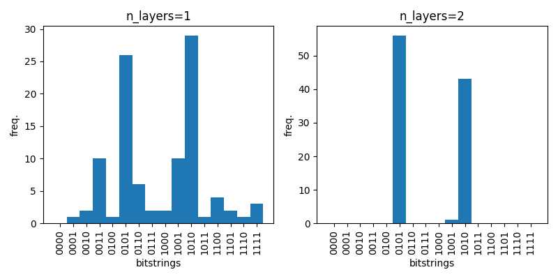
Plotting the results

We can plot the distribution of measurements obtained from the optimized circuits. As expected for this graph, the partitions 0101 and 1010 are measured with the highest frequencies, and in the case where we set n_layers=2 we obtain one of the optimal partitions with 100% certainty.

import matplotlib.pyplot as plt

xticks = range(0, 16)
xtick_labels = list(map(lambda x: format(x, "04b"), xticks))
bins = np.arange(0, 17) - 0.5

fig, (ax1, ax2) = plt.subplots(1, 2, figsize=(8, 4))
plt.subplot(1, 2, 1)
plt.title("n_layers=1")
plt.xlabel("bitstrings")
plt.ylabel("freq.")
plt.xticks(xticks, xtick_labels, rotation="vertical")
plt.hist(bitstrings1, bins=bins)
plt.subplot(1, 2, 2)
plt.title("n_layers=2")
plt.xlabel("bitstrings")
plt.ylabel("freq.")
plt.xticks(xticks, xtick_labels, rotation="vertical")
plt.hist(bitstrings2, bins=bins)
plt.tight_layout()
plt.show()

About the author

Angus Lowe

Angus is currently a PhD student in physics at the Massachusetts Institute of Technology. His main research interests are in the theory of quantum computation and quantum information.

demos/tutorial_qaoa_maxcut

 

Download Python script

 

Download Notebook

 

View on GitHub