Note
Click here to download the full example code
Kernel-based training of quantum models with scikit-learn
Author: Maria Schuld — Posted: 03 February 2021. Last updated: 3 February 2021.
Over the last few years, quantum machine learning research has provided a lot of insights on how we can understand and train quantum circuits as machine learning models. While many connections to neural networks have been made, it becomes increasingly clear that their mathematical foundation is intimately related to so-called kernel methods, the most famous of which is the support vector machine (SVM) (see for example Schuld and Killoran (2018), Havlicek et al. (2018), Liu et al. (2020), Huang et al. (2020), and, for a systematic summary which we will follow here, Schuld (2021)).
The link between quantum models and kernel methods has important practical implications: we can replace the common variational approach to quantum machine learning with a classical kernel method where the kernel—a small building block of the overall algorithm—is computed by a quantum device. In many situations there are guarantees that we get better or at least equally good results.
This demonstration explores how kernel-based training compares with variational training in terms of the number of quantum circuits that have to be evaluated. For this we train a quantum machine learning model with a kernel-based approach using a combination of PennyLane and the scikit-learn machine learning library. We compare this strategy with a variational quantum circuit trained via stochastic gradient descent using PyTorch.
We will see that in a typical small-scale example, kernel-based training requires only a fraction of the number of quantum circuit evaluations used by variational circuit training, while each evaluation runs a much shorter circuit. In general, the relative efficiency of kernel-based methods compared to variational circuits depends on the number of parameters used in the variational model.
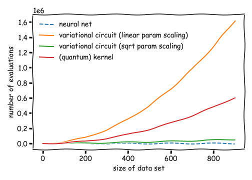
If the number of variational parameters remains small, e.g., there is a square-root-like scaling with the number of data samples (green line), variational circuits are almost as efficient as neural networks (blue line), and require much fewer circuit evaluations than the quadratic scaling of kernel methods (red line). However, with current hardware-compatible training strategies, kernel methods scale much better than variational circuits that require a number of parameters of the order of the training set size (orange line).
In conclusion, for quantum machine learning applications with many parameters, kernel-based training can be a great alternative to the variational approach to quantum machine learning.
After working through this demo, you will:
be able to use a support vector machine with a quantum kernel computed with PennyLane, and
be able to compare the scaling of quantum circuit evaluations required in kernel-based versus variational training.
Background
Let us consider a quantum model of the form
where \(| \phi(x)\rangle\) is prepared by a fixed embedding circuit that encodes data inputs \(x\), and \(\mathcal{M}\) is an arbitrary observable. This model includes variational quantum machine learning models, since the observable can effectively be implemented by a simple measurement that is preceded by a variational circuit:
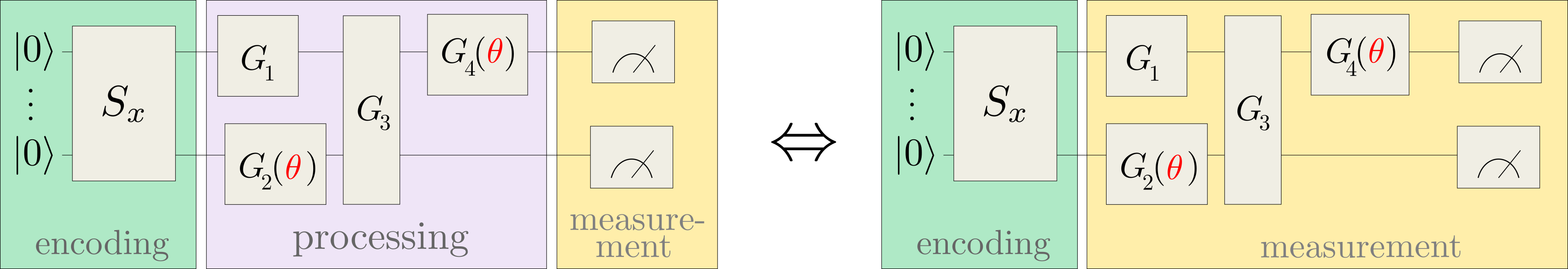
For example, applying a circuit \(G(\theta)\) and then measuring the Pauli-Z observable \(\sigma^0_z\) of the first qubit implements the trainable measurement \(\mathcal{M}(\theta) = G^{\dagger}(\theta) \sigma^0_z G(\theta)\).
The main practical consequence of approaching quantum machine learning with a kernel approach is that instead of training \(f\) variationally, we can often train an equivalent classical kernel method with a kernel executed on a quantum device. This quantum kernel is given by the mutual overlap of two data-encoding quantum states,
Kernel-based training therefore bypasses the processing and measurement parts of common variational circuits, and only depends on the data encoding.
If the loss function \(L\) is the hinge loss, the kernel method corresponds to a standard support vector machine (SVM) in the sense of a maximum-margin classifier. Other convex loss functions lead to more general variations of support vector machines.
Note
More precisely, we can replace variational with kernel-based training if the optimisation problem can be written as minimizing a cost of the form
which is a regularized empirical risk with training data samples \((x^m, y^m)_{m=1\dots M}\), regularization strength \(\lambda \in \mathbb{R}\), and loss function \(L\).
Theory predicts that kernel-based training will always find better or equally good minima of this risk. However, to show this here we would have to either regularize the variational training by the trace of the squared observable, or switch off regularization in the classical SVM, which removes a lot of its strength. The kernel-based and the variational training in this demonstration therefore optimize slightly different cost functions, and it is out of our scope to establish whether one training method finds a better minimum than the other.
Kernel-based training
First, we will turn to kernel-based training of quantum models. As stated above, an example implementation is a standard support vector machine with a kernel computed by a quantum circuit.
We begin by importing all sorts of useful methods:
import numpy as np
import torch
from torch.nn.functional import relu

from sklearn.svm import SVC
from sklearn.datasets import load_iris
from sklearn.preprocessing import StandardScaler
from sklearn.model_selection import train_test_split
from sklearn.metrics import accuracy_score

import pennylane as qml
from pennylane.templates import AngleEmbedding, StronglyEntanglingLayers
from pennylane.operation import Tensor

import matplotlib.pyplot as plt

np.random.seed(42)
The second step is to define a data set. Since the performance of the models is not the focus of this demo, we can just use the first two classes of the famous Iris data set. Dating back to as far as 1936, this toy data set consists of 100 samples of four features each, and gives rise to a very simple classification problem.
X, y = load_iris(return_X_y=True)

# pick inputs and labels from the first two classes only,
# corresponding to the first 100 samples
X = X[:100]
y = y[:100]

# scaling the inputs is important since the embedding we use is periodic
scaler = StandardScaler().fit(X)
X_scaled = scaler.transform(X)

# scaling the labels to -1, 1 is important for the SVM and the
# definition of a hinge loss
y_scaled = 2 * (y - 0.5)

X_train, X_test, y_train, y_test = train_test_split(X_scaled, y_scaled)
We use the angle-embedding template which needs as many qubits as there are features:
n_qubits = len(X_train[0])
n_qubits
Out:
4
To implement the kernel we could prepare the two states \(| \phi(x) \rangle\), \(| \phi(x') \rangle\) on different sets of qubits with angle-embedding routines \(S(x), S(x')\), and measure their overlap with a small routine called a SWAP test.
However, we need only half the number of qubits if we prepare \(| \phi(x)\rangle\) and then apply the inverse embedding with \(x'\) on the same qubits. We then measure the projector onto the initial state \(|0..0\rangle \langle 0..0|\).
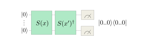
To verify that this gives us the kernel:
Note that a projector \(|0..0 \rangle \langle 0..0|\) can be constructed
using the qml.Hermitian observable in PennyLane.
Altogether, we use the following quantum node as a quantum kernel evaluator:
dev_kernel = qml.device("default.qubit", wires=n_qubits)

projector = np.zeros((2**n_qubits, 2**n_qubits))
projector[0, 0] = 1

@qml.qnode(dev_kernel, interface="autograd")
def kernel(x1, x2):
    """The quantum kernel."""
    AngleEmbedding(x1, wires=range(n_qubits))
    qml.adjoint(AngleEmbedding)(x2, wires=range(n_qubits))
    return qml.expval(qml.Hermitian(projector, wires=range(n_qubits)))
A good sanity check is whether evaluating the kernel of a data point and itself returns 1:
kernel(X_train[0], X_train[0])
Out:
tensor(1., requires_grad=True)
The way an SVM with a custom kernel is implemented in scikit-learn requires us to pass a function that computes a matrix of kernel evaluations for samples in two different datasets A, B. If A=B, this is the Gram matrix.
def kernel_matrix(A, B):
    """Compute the matrix whose entries are the kernel
       evaluated on pairwise data from sets A and B."""
    return np.array([[kernel(a, b) for b in B] for a in A])
Training the SVM optimizes internal parameters that basically weigh kernel functions. It is a breeze in scikit-learn, which is designed as a high-level machine learning library:
svm = SVC(kernel=kernel_matrix).fit(X_train, y_train)
Let’s compute the accuracy on the test set.
predictions = svm.predict(X_test)
accuracy_score(predictions, y_test)
Out:
1.0
The SVM predicted all test points correctly. How many times was the quantum device evaluated?
Out:
7501
This number can be derived as follows: For \(M\) training samples, the SVM must construct the \(M \times M\) dimensional kernel gram matrix for training. To classify \(M_{\rm pred}\) new samples, the SVM needs to evaluate the kernel at most \(M_{\rm pred}M\) times to get the pairwise distances between training vectors and test samples.
Note
Depending on the implementation of the SVM, only \(S \leq M_{\rm pred}\) support vectors are needed.
Let us formulate this as a function, which can be used at the end of the demo to construct the scaling plot shown in the introduction.
def circuit_evals_kernel(n_data, split):
    """Compute how many circuit evaluations one needs for kernel-based
       training and prediction."""

    M = int(np.ceil(split * n_data))
    Mpred = n_data - M

    n_training = M * M
    n_prediction = M * Mpred

    return n_training + n_prediction
With \(M = 75\) and \(M_{\rm pred} = 25\), the number of kernel evaluations can therefore be estimated as:
circuit_evals_kernel(n_data=len(X), split=len(X_train) /(len(X_train) + len(X_test)))
Out:
7500
The single additional evaluation can be attributed to evaluating the kernel once above as a sanity check.
A similar example using variational training
Using the variational principle of training, we can propose an ansatz for the variational circuit and train it directly. By increasing the number of layers of the ansatz, its expressivity increases. Depending on the ansatz, we may only search through a subspace of all measurements for the best candidate.
Remember from above, the variational training does not optimize exactly the same cost as the SVM, but we try to match them as closely as possible. For this we use a bias term in the quantum model, and train on the hinge loss.
We also explicitly use the parameter-shift
differentiation method in the quantum node, since this is a method which works on hardware as well.
While diff_method='backprop' or diff_method='adjoint' would reduce the number of
circuit evaluations significantly, they are based on tricks that are only suitable for simulators,
and can therefore not scale to more than a few dozen qubits.
dev_var = qml.device("default.qubit", wires=n_qubits)

@qml.qnode(dev_var, interface="torch", diff_method="parameter-shift")
def quantum_model(x, params):
    """A variational quantum model."""

    # embedding
    AngleEmbedding(x, wires=range(n_qubits))

    # trainable measurement
    StronglyEntanglingLayers(params, wires=range(n_qubits))
    return qml.expval(qml.PauliZ(0))

def quantum_model_plus_bias(x, params, bias):
    """Adding a bias."""
    return quantum_model(x, params) + bias

def hinge_loss(predictions, targets):
    """Implements the hinge loss."""
    all_ones = torch.ones_like(targets)
    hinge_loss = all_ones - predictions * targets
    # trick: since the max(0,x) function is not differentiable,
    # use the mathematically equivalent relu instead
    hinge_loss = relu(hinge_loss)
    return hinge_loss
We now summarize the usual training and prediction steps into two
functions similar to scikit-learn’s fit() and predict(). While
it feels cumbersome compared to the one-liner used to train the kernel method,
PennyLane—like other differentiable programming libraries—provides a lot more
control over the particulars of training.
In our case, most of the work is to convert between numpy and torch,
which we need for the differentiable relu function used in the hinge loss.
def quantum_model_train(n_layers, steps, batch_size):
    """Train the quantum model defined above."""

    params = np.random.random((n_layers, n_qubits, 3))
    params_torch = torch.tensor(params, requires_grad=True)
    bias_torch = torch.tensor(0.0)

    opt = torch.optim.Adam([params_torch, bias_torch], lr=0.1)

    loss_history = []
    for i in range(steps):

        batch_ids = np.random.choice(len(X_train), batch_size)

        X_batch = X_train[batch_ids]
        y_batch = y_train[batch_ids]

        X_batch_torch = torch.tensor(X_batch, requires_grad=False)
        y_batch_torch = torch.tensor(y_batch, requires_grad=False)

        def closure():
            opt.zero_grad()
            preds = torch.stack(
                [quantum_model_plus_bias(x, params_torch, bias_torch) for x in X_batch_torch]
            )
            loss = torch.mean(hinge_loss(preds, y_batch_torch))

            # bookkeeping
            current_loss = loss.detach().numpy().item()
            loss_history.append(current_loss)
            if i % 10 == 0:
                print("step", i, ", loss", current_loss)

            loss.backward()
            return loss

        opt.step(closure)

    return params_torch, bias_torch, loss_history


def quantum_model_predict(X_pred, trained_params, trained_bias):
    """Predict using the quantum model defined above."""

    p = []
    for x in X_pred:

        x_torch = torch.tensor(x)
        pred_torch = quantum_model_plus_bias(x_torch, trained_params, trained_bias)
        pred = pred_torch.detach().numpy().item()
        if pred > 0:
            pred = 1
        else:
            pred = -1

        p.append(pred)
    return p
Let’s train the variational model and see how well we are doing on the test set.
n_layers = 2
batch_size = 20
steps = 100
trained_params, trained_bias, loss_history = quantum_model_train(n_layers, steps, batch_size)
pred_test = quantum_model_predict(X_test, trained_params, trained_bias)
print("accuracy on test set:", accuracy_score(pred_test, y_test))
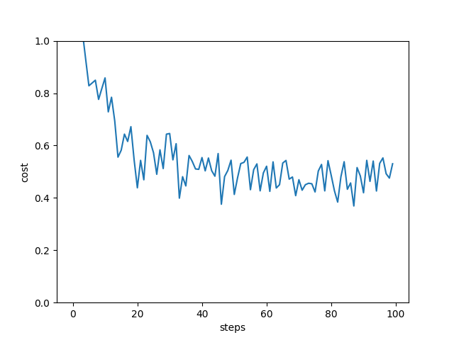
plt.plot(loss_history)
plt.ylim((0, 1))
plt.xlabel("steps")
plt.ylabel("cost")
plt.show()
Out:
step 0 , loss 1.2128428849025235
step 10 , loss 0.8582750956106432
step 20 , loss 0.4384989057963328
step 30 , loss 0.6458829274590644
step 40 , loss 0.5540116701446125
step 50 , loss 0.4132239145818263
step 60 , loss 0.5209433003814096
step 70 , loss 0.4694193423160378
step 80 , loss 0.4858145744021137
step 90 , loss 0.41962346215340257
accuracy on test set: 0.96
The variational circuit has a slightly lower accuracy than the SVM—but this depends very much on the training settings we used. Different random parameter initializations, more layers, or more steps may indeed get perfect test accuracy.
How often was the device executed?
Out:
74025
That is a lot more than the kernel method took!
Let’s try to understand this value. In each optimization step, the variational circuit needs to compute the partial derivative of all trainable parameters for each sample in a batch. Using parameter-shift rules, we require roughly two circuit evaluations per partial derivative. Prediction uses only one circuit evaluation per sample.
We can formulate this as another function that will be used in the scaling plot below.
def circuit_evals_variational(n_data, n_params, n_steps, shift_terms, split, batch_size):
    """Compute how many circuit evaluations are needed for
       variational training and prediction."""

    M = int(np.ceil(split * n_data))
    Mpred = n_data - M

    n_training = n_params * n_steps * batch_size * shift_terms
    n_prediction = Mpred

    return n_training + n_prediction
This estimates the circuit evaluations in variational training as:
circuit_evals_variational(
    n_data=len(X),
    n_params=len(trained_params.flatten()),
    n_steps=steps,
    shift_terms=2,
    split=len(X_train) /(len(X_train) + len(X_test)),
    batch_size=batch_size,
)
Out:
96025
The estimate is a bit higher because it does not account for some optimizations that PennyLane performs under the hood.
It is important to note that while they are trained in a similar manner, the number of variational circuit evaluations differs from the number of neural network model evaluations in classical machine learning, which would be given by:
def model_evals_nn(n_data, n_params, n_steps, split, batch_size):
    """Compute how many model evaluations are needed for neural
       network training and prediction."""

    M = int(np.ceil(split * n_data))
    Mpred = n_data - M

    n_training = n_steps * batch_size
    n_prediction = Mpred

    return n_training + n_prediction
In each step of neural network training, and due to the clever implementations of automatic differentiation,
the backpropagation algorithm can compute a
gradient for all parameters in (more-or-less) a single run.
For all we know at this stage, the no-cloning principle prevents variational circuits from using these tricks,
which leads to n_training in circuit_evals_variational depending on the number of parameters, but not in
model_evals_nn.
For the same example as used here, a neural network would therefore have far fewer model evaluations than both variational and kernel-based training:
model_evals_nn(
    n_data=len(X),
    n_params=len(trained_params.flatten()),
    n_steps=steps,
    split=len(X_train) /(len(X_train) + len(X_test)),
    batch_size=batch_size,
)
Out:
2025
Which method scales best?
The answer to this question depends on how the variational model is set up, and we need to make a few assumptions:
Even if we use single-batch stochastic gradient descent, in which every training step uses exactly one training sample, we would want to see every training sample at least once on average. Therefore, the number of steps should scale at least linearly with the number of training data samples.
Modern neural networks often have many more parameters than training samples. But we do not know yet whether variational circuits really need that many parameters as well. We will therefore use two cases for comparison:
2a) the number of parameters grows linearly with the training data, or
n_params = M,2b) the number of parameters saturates at some point, which we model by setting
n_params = sqrt(M).
Note that compared to the example above with 75 training samples and 24 parameters, a) overestimates the number of evaluations, while b) underestimates it.
This is how the three methods compare:
variational_training1 = []
variational_training2 = []
kernelbased_training = []
nn_training = []
x_axis = range(0, 2000, 100)

for M in x_axis:

    var1 = circuit_evals_variational(
        n_data=M, n_params=M, n_steps=M,  shift_terms=2, split=0.75, batch_size=1
    )
    variational_training1.append(var1)

    var2 = circuit_evals_variational(
        n_data=M, n_params=round(np.sqrt(M)), n_steps=M,
        shift_terms=2, split=0.75, batch_size=1
    )
    variational_training2.append(var2)

    kernel = circuit_evals_kernel(n_data=M, split=0.75)
    kernelbased_training.append(kernel)

    nn = model_evals_nn(
        n_data=M, n_params=M, n_steps=M, split=0.75, batch_size=1
    )
    nn_training.append(nn)


plt.plot(x_axis, nn_training, linestyle='--', label="neural net")
plt.plot(x_axis, variational_training1, label="var. circuit (linear param scaling)")
plt.plot(x_axis, variational_training2, label="var. circuit (srqt param scaling)")
plt.plot(x_axis, kernelbased_training, label="(quantum) kernel")
plt.xlabel("size of data set")
plt.ylabel("number of evaluations")
plt.legend()
plt.tight_layout()
plt.show()
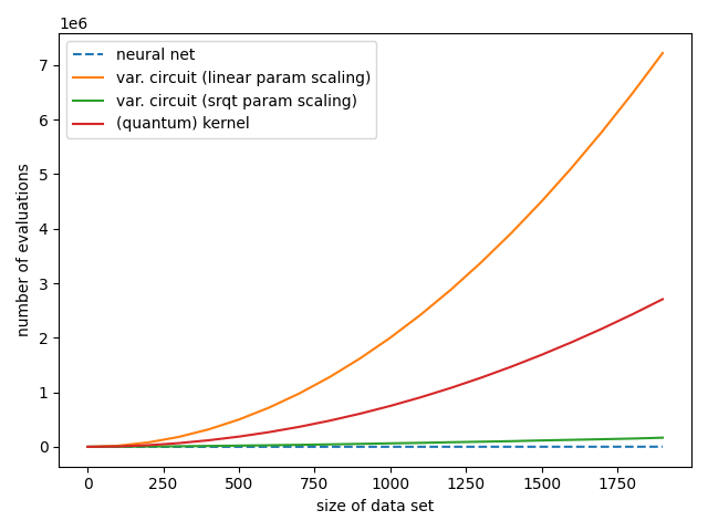
This is the plot we saw at the beginning. With current hardware-compatible training methods, whether kernel-based training requires more or fewer quantum circuit evaluations than variational training depends on how many parameters the latter needs. If variational circuits turn out to be as parameter-hungry as neural networks, kernel-based training will outperform them for common machine learning tasks. However, if variational learning only turns out to require few parameters (or if more efficient training methods are found), variational circuits could in principle match the linear scaling of neural networks trained with backpropagation.
The practical take-away from this demo is that unless your variational circuit has significantly fewer parameters than training data, kernel methods could be a much faster alternative!
Finally, it is important to note that fault-tolerant quantum computers may change the picture for both quantum and classical machine learning. As mentioned in Schuld (2021), early results from the quantum machine learning literature show that larger quantum computers will most likely enable us to reduce the quadratic scaling of kernel methods to linear scaling, which may make classical as well as quantum kernel methods a strong alternative to neural networks for big data processing one day.