Measurement-based quantum computation

Authors: Joost Bus and Radoica Draškić — Posted: 05 December 2022. Last updated: 05 December 2022.

Measurement-based quantum computing (MBQC), also known as one-way quantum computing, is an inventive approach to quantum computing that makes use of off-line entanglement as a resource for computation. A one-way quantum computer starts out with an entangled state, a so-called cluster state, and applies particular single-qubit measurements that correspond to the desired quantum circuit. In this context, off-line means that the entanglement is created independently from the rest of the computation, like how a blank sheet of paper is made separately from the text of a book. Coming from the gate-based model, this method might seem unintuitive to you at first, but the approaches can be proven to be equally powerful. In MBQC, the measurements are the computation and the entanglement of the cluster state is used as a resource.

The structure of this demo will be as follows. First, we introduce the concept of a cluster state, the substrate for measurement-based quantum computation. Then, we will move on to explain how to implement arbitrary quantum circuits, thus proving that MBQC is universal. Lastly, we will briefly touch upon how quantum error correction (QEC) is done in this scheme.

Throughout this tutorial, we will explain the underlying concepts with the help of some code snippets using PennyLane. In the section about QEC, we will also use Xanadu’s quantum error correction simulation software FlamingPy developed by our architecture team 4.

In MBQC, seeing is computing!

Cluster states and graph states

Cluster states are the universal substrate for measurement-based quantum computation 1. They are a special instance of graph states 20, a class of entangled multi-qubit states that can be represented by an undirected graph \(G = (V,E)\) whose vertices \(V\) are associated with qubits and the edges \(E\) with entanglement between them. The associated quantum state reads as follows

\[|\Phi\rangle=\Pi_{(i,j)\in E}CZ_{ij}|+⟩^{\otimes n}.\]

where \(n\) is the number of qubits, \(CZ_{ij}\) is the controlled-\(Z\) gate between qubits \(i\) and \(j\), and \(|+\rangle = \frac{1}{\sqrt{2}}\big(|0\rangle + |1\rangle\big)\) is the \(+1\) eigenstate of the Pauli-\(X\) operator. The distinction between graph states and a cluster states is rather technical and details can be found in Ref. 21. For now, suffice to say that cluster states are a subset of graph states with some additional conditions.

We can also describe the creation of a cluster state in the gate-based model. Let us first define a graph we want to look at, and then construct a circuit in PennyLane to create the corresponding graph state.

import networkx as nx
import matplotlib.pyplot as plt

a, b = 1, 5  # dimensions of the graph (lattice)
G = nx.grid_graph(dim=[a, b])  # there are a * b qubits

plt.figure(figsize=(5, 1))
nx.draw(G, pos={node: node for node in G}, node_size=500, node_color="black")

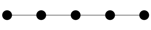
This is a fairly simple cluster state, but we will later see how even this simple graph is useful for logical operations. Now that we have defined a graph, we can go ahead and define a circuit to prepare the cluster state.

import pennylane as qml

qubits = [str(node) for node in G.nodes]
dev = qml.device("default.qubit", wires=qubits)


@qml.qnode(dev, interface="autograd")
def cluster_state():
    for node in qubits:
        qml.Hadamard(wires=[node])

    for edge in G.edges:
        i, j = edge
        qml.CZ(wires=[str(i), str(j)])

    return qml.state()


print(qml.draw(cluster_state)())

Out:

(0, 0): ──H─╭●──────────┤  State
(1, 0): ──H─╰Z─╭●───────┤  State
(2, 0): ──H────╰Z─╭●────┤  State
(3, 0): ──H───────╰Z─╭●─┤  State
(4, 0): ──H──────────╰Z─┤  State

Observe that the structure of the circuit is fairly simple. It only requires Hadamard gates on each qubit and then a controlled-\(Z\) gate between connected qubits. This part of the computation is not actually computing anything. In fact, aside from the width and depth of the desired quantum circuit, the cluster state generation is essentially independent of the calculation. If you have a reliable way of applying these two operations (Hadamard and controlled-\(Z\)), you are ready for the next step: worrying about conditional single-qubit measurements.

Information propagation and teleportation

Measurement-based quantum computation heavily relies on the idea of information propagation. In particular, we make use of a protocol called quantum teleportation, one of the driving concepts behind MBQC. Despite its Sci-Fi name, quantum teleportation is very real and has been experimentally demonstrated multiple times in the last few decades 13, 11, 14, 12. Moreover, it has related applications in safe communication protocols that are impossible with classical communication so it’s certainly worth learning about. In this protocol, we transport information, not matter, between systems. Admittedly, it has a somewhat misleading name because it is not instantaneous: it requires communication of additional classical information, which is still limited by the speed of light.

One-qubit Teleportation

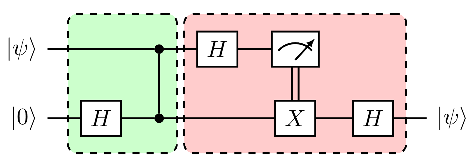
Let’s take a deeper look at the principles behind quantum teleportation using a simple example of one-qubit teleportation. We start with one qubit in the state \(|\psi\rangle\) that we want to transfer to the second qubit initially in the state \(|0\rangle\). The figure below represents the protocol. The green box represents the creation of a cluster state, while the red box represents the measurement of a qubit with the appropriate correction applied to the second qubit based on the measurement outcome.

Let’s implement one-qubit teleportation in PennyLane.

import pennylane as qml
import pennylane.numpy as np

dev = qml.device("default.qubit", wires=2)


@qml.qnode(dev, interface="autograd")
def one_bit_teleportation(input_state):
    # Prepare the input state
    qml.QubitStateVector(input_state, wires=0)

    # Prepare the cluster state
    qml.Hadamard(wires=1)
    qml.CZ(wires=[0, 1])

    # Measure the first qubit in the Pauli-X basis
    # and apply an X-gate conditioned on the outcome
    qml.Hadamard(wires=0)
    m = qml.measure(wires=[0])
    qml.cond(m == 1, qml.PauliX)(wires=1)
    qml.Hadamard(wires=1)

    # Return the density matrix of the output state
    return qml.density_matrix(wires=[1])

Note that we return a density matrix in the function above. This allows for us to describe operations beyond unitaries, such as the teleportation protocol.

Now, let’s prepare a random qubit state and see if the teleportation protocol is working as expected. To do so, we’ll generate a random normalized state \(|\psi\rangle = \alpha |0\rangle + \beta |1\rangle\) and apply the teleportation protocol to see if the resulting density matrix describing the second qubit is the same as our input state \(|\psi\rangle\).

# Define helper function for random input state on n qubits
def generate_random_state(n=1):
    input_state = np.random.random(2 ** n) + 1j * np.random.random(2 ** n)
    return input_state / np.linalg.norm(input_state)


# Generate a random input state |psi> for n=1 qubit
input_state = generate_random_state()

density_matrix = np.outer(input_state, np.conj(input_state))
density_matrix_mbqc = one_bit_teleportation(input_state)

np.allclose(density_matrix, density_matrix_mbqc)

Out:

True

As we can see, \(|\psi\rangle\), originally the state of the first qubit, has been transported to the second qubit!

This protocol is one of the main ingredients of one-way quantum computing. Essentially, we propagate the information in one end of our cluster state to the other end through successive teleportations. In addition, we can “write” our circuit onto the cluster state by choosing the measurements adaptively. In the next section, we will see how we can actually do this.

Universality of MBQC

How do we know if this measurement-based scheme is just as powerful as its gate-based counterpart? We have to prove it! In particular, we want to show that a measurement-based quantum computer is a quantum Turing machine (QTM). To do this, we need to show 4 things 1:

1. How information propagates through the cluster state.

2. How arbitrary single-qubit rotations can be implemented.

3. How a two-qubit gate can be implemented in this scheme.

4. How to implement arbitrary quantum circuits.

In the previous section, we have already seen how the quantum information propagates from one side of the cluster to the other. In this section, we will tackle the remaining parts concerning logical operations. Throughout, we will assume the ability to measure in arbitrary bases.

Single-qubit rotations

Arbitrary single-qubit rotations are essential operations for a universal quantum computer. In MBQC, we can implement these rotations by using the entanglement of the cluster state. Any single-qubit gate can be represented as a composition of three rotations along two different axes, for example \(U(\alpha, \beta, \gamma) = R_x(\gamma)R_z(\beta)R_x(\alpha)\) where \(R_x\) and \(R_z\) represent rotations around the \(X\) and \(Z\) axis, respectively.

We will see that in our measurement-based scheme, this operation can be implemented using a linear chain of 5 qubits prepared in a cluster state, as shown in the figure below 2. The first qubit \(t_\mathrm{in}\) is prepared in some input state \(|\psi_\mathrm{in}\rangle\), and we are interested in the final state of the output qubit \(t_\mathrm{out}\).

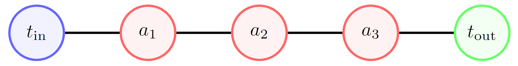
The input qubit \(t_\mathrm{in}\), together with the intermediate qubits \(a_1\), \(a_2\), and \(a_3\) are then measured in the bases

\[\mathcal{B}_j(\theta_j) \equiv \left\{\frac{|0\rangle + e^{i\theta_j}|1\rangle}{\sqrt{2}}, \frac{|0\rangle - e^{i\theta_j}|1\rangle}{\sqrt{2}}\right\},\]

where the angles \(\theta_j\) depend on prior measurement outcomes and are given by

\[\theta_{\mathrm{in}} = 0, \qquad \theta_{1} = (-1)^{m_{\mathrm{in}} + 1} \alpha, \qquad \theta_{2} = (-1)^{m_1} \beta, \quad \text{and} \quad \theta_{3} = (-1)^{m_{\mathrm{in}} + m_2} \gamma\]

with \(m_{\mathrm{in}}, m_1, m_2 \in \{0, 1\}\) being the measurement outcomes on nodes \(t_\mathrm{in}\), \(a_1\) and \(a_2\), respectively. Note that the measurement basis is adaptive; the measurement on \(a_3\), for example, depends on the outcome of earlier measurements in the chain. After these operations, the state of qubit \(t_\mathrm{out}\) is given by

\[|\psi_{\mathrm{out}}\rangle = \tilde{U}(\alpha, \beta, \gamma)|\psi_{\mathrm{in}}\rangle = X^{m_1 + m_3}Z^{m_{\mathrm{in}} + m_2}U(\alpha, \beta, \gamma) |\psi_{\mathrm{in}}\rangle.\]

with \(m_3\) being the measurement outcome on node \(a_3\). Now note that this unitary \(\tilde{U}\) is related to our desired unitary \(U\) up to the first two Pauli terms. Luckily, we can correct for these additional Pauli gates by choosing the measurement basis of qubit \(t_\mathrm{out}\) appropriately or correcting for them classically after the quantum computation.

To demonstrate that this actually works, we will use PennyLane. For simplicity, we will just show the ability will to perform single-axis rotations \(R_z(\theta)\) and \(R_x(\theta)\) for arbitrary \(\theta \in [0, 2 \pi)\). Note that these two operations plus the CNOT also constitute a universal gate set.

To start off, we define the \(R_z(\theta)\) gate using two qubits with the gate-based approach so we can later compare our MBQC approach to it.

dev = qml.device("default.qubit", wires=1)


@qml.qnode(dev, interface="autograd")
def RZ(theta, input_state):
    # Prepare the input state
    qml.QubitStateVector(input_state, wires=0)

    # Perform the Rz rotation
    qml.RZ(theta, wires=0)

    # Return the density matrix of the output state
    return qml.density_matrix(wires=[0])

Let’s now implement an \(R_z\) gate on an arbitrary state in the MBQC formalism.

mbqc_dev = qml.device("default.qubit", wires=2)


@qml.qnode(mbqc_dev, interface="autograd")
def RZ_MBQC(theta, input_state):
    # Prepare the input state
    qml.QubitStateVector(input_state, wires=0)

    # Prepare the cluster state
    qml.Hadamard(wires=1)
    qml.CZ(wires=[0, 1])

    # Measure the first qubit an correct the state
    qml.RZ(theta, wires=0)
    qml.Hadamard(wires=0)
    m = qml.measure(wires=[0])

    qml.cond(m == 1, qml.PauliX)(wires=1)
    qml.Hadamard(wires=1)

    # Return the density matrix of the output state
    return qml.density_matrix(wires=[1])

Next, we will prepare a random input state and compare the two approaches.

# Generate a random input state
input_state = generate_random_state()
theta = 2 * np.pi * np.random.random()

np.allclose(RZ(theta, input_state), RZ_MBQC(theta, input_state))

Out:

True

Seems good! As we can see, the resulting states are practically the same. For the \(R_x(\theta)\) gate we take a similar approach.

dev = qml.device("default.qubit", wires=1)


@qml.qnode(dev, interface="autograd")
def RX(theta, input_state):
    # Prepare the input state
    qml.QubitStateVector(input_state, wires=0)

    # Perform the Rz rotation
    qml.RX(theta, wires=0)

    # Return the density matrix of the output state
    return qml.density_matrix(wires=[0])


mbqc_dev = qml.device("default.qubit", wires=3)


@qml.qnode(mbqc_dev, interface="autograd")
def RX_MBQC(theta, input_state):
    # Prepare the input state
    qml.QubitStateVector(input_state, wires=0)

    # Prepare the cluster state
    qml.Hadamard(wires=1)
    qml.Hadamard(wires=2)
    qml.CZ(wires=[0, 1])
    qml.CZ(wires=[1, 2])

    # Measure the qubits and perform corrections
    qml.Hadamard(wires=0)
    m1 = qml.measure(wires=[0])

    qml.RZ(theta, wires=1)
    qml.cond(m1 == 1, qml.RX)(-2 * theta, wires=2)
    qml.Hadamard(wires=1)
    m2 = qml.measure(wires=[1])

    qml.cond(m2 == 1, qml.PauliX)(wires=2)
    qml.cond(m1 == 1, qml.PauliZ)(wires=2)

    # Return the density matrix of the output state
    return qml.density_matrix(wires=[2])

Finally, we again compare the two implementations with a random state as an input.

# Generate a random input state
input_state = generate_random_state()
theta = 2 * np.pi * np.random.random()

np.allclose(RX(theta, input_state), RX_MBQC(theta, input_state))

Out:

True

Perfect! We have shown that we can implement any single-axis rotation on an arbitrary state in the MBQC formalism. In the following section we will look at a two-qubit gate to complete our universal gate set.

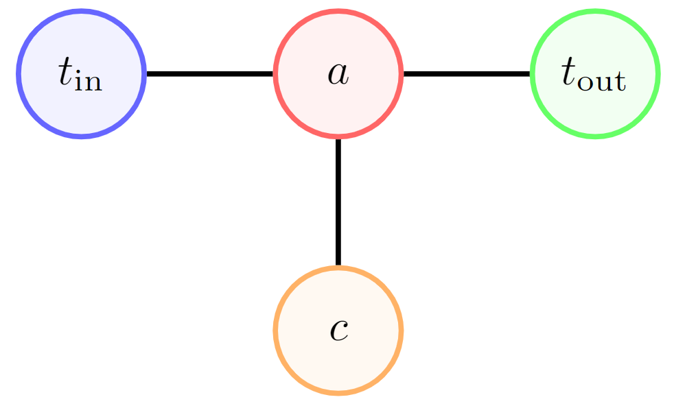
The two-qubit gate: CNOT

The second ingredient for a universal quantum computing scheme is the two-qubit gate. Here, we will show how to perform a CNOT operation in the measurement-based framework. The input state is given on two qubits, control qubit \(c\) and target qubit \(t_\mathrm{in}\). Preparing the cluster state shown in the figure below, and measuring qubits \(t_\mathrm{in}\) and \(a\) in the \(X\)-basis, we implement the CNOT gate between qubits \(c\) and \(t_\mathrm{out}\) up to Pauli corrections 2.

Let’s see how one can do this in PennyLane.

dev = qml.device("default.qubit", wires=2)


@qml.qnode(dev, interface="autograd")
def CNOT(input_state):
    # Prepare the input state
    qml.QubitStateVector(input_state, wires=[0, 1])
    qml.CNOT(wires=[0, 1])

    return qml.density_matrix(wires=[0, 1])


mbqc_dev = qml.device("default.qubit", wires=4)


@qml.qnode(mbqc_dev, interface="autograd")
def CNOT_MBQC(input_state):
    # Prepare the input state
    qml.QubitStateVector(input_state, wires=[0, 1])

    # Prepare the cluster state
    qml.Hadamard(wires=2)
    qml.Hadamard(wires=3)
    qml.CZ(wires=[2, 0])
    qml.CZ(wires=[2, 1])
    qml.CZ(wires=[2, 3])

    # Measure the qubits in the appropriate bases
    qml.Hadamard(wires=1)
    m1 = qml.measure(wires=[1])
    qml.Hadamard(wires=2)
    m2 = qml.measure(wires=[2])

    # Correct the state
    qml.cond(m1 == 1, qml.PauliZ)(wires=0)
    qml.cond(m2 == 1, qml.PauliX)(wires=3)
    qml.cond(m1 == 1, qml.PauliZ)(wires=3)

    # Return the density matrix of the output state
    return qml.density_matrix(wires=[0, 3])

Now let’s prepare a random input state and check our implementation.

# Generate a random 2-qubit state
input_state = generate_random_state(n=2)

np.allclose(CNOT(input_state), CNOT_MBQC(input_state))

Out:

True

Arbitrary quantum circuits

Once we have established the ability to implement arbitrary single-qubit rotations and a two-qubit gate, the final step is to show that we can implement arbitrary quantum circuits. To do so, we simply have to note that we have a universal gate set 10. The complete computation can be performed as shown in the figure below. The qubits are teleported along the arrows in the cluster and single-qubit gates are applied through a selection of measurement bases along these arrays. Two-qubit gates are implemented along vertical arrows, and the rest of the qubits are measured in the \(Z\)-basis, effectively taking them out of the cluster without affecting the neighboring nodes.

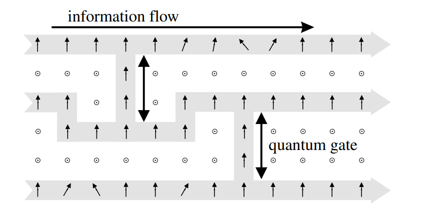
A complete measurement-based quantum computation. Circles \(\odot\) symbolize measurements of Pauli-\(Z\), vertical arrows \(\uparrow\) are measurements of Pauli-\(X\), while tilted arrows \(\nwarrow\) or \(\nearrow\) refer to measurements in the \(xy\)-plane. 1

However, you might wonder: Is it even feasible to construct the large cluster states that one-way quantum computation requires? The number of qubits needed to construct a circuit can grow to be very large, as it not only depends on the number of logical qubits, but also on the depth of the circuit. At this point, it’s good to reiterate that the entanglement of the cluster state is created off-line.

…the entanglement is created independently from the rest of the computation, like how a blank sheet of paper is made separately from the text of a book.

Interestingly enough, we do not have to prepare all of the entanglement at once. Just like we can already start printing text upon the first few pages, we can apply measurements to one end of the cluster while growing it at the same time, as shown in the figure below. That is, we can start printing the text on the first few pages while at the same time reloading the printer’s paper tray!

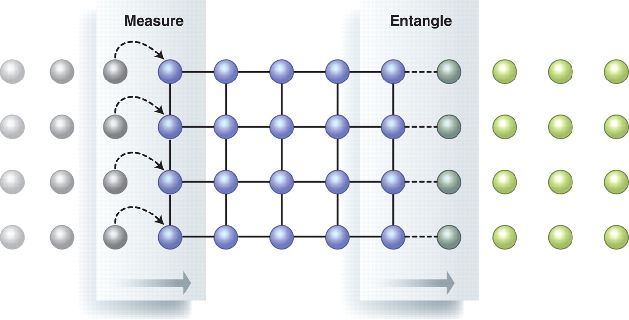
Schematic showing how we can also consume the cluster state while we grow it. The blue qubits are in a cluster state, where the bonds between them represent entanglement. The gray qubits have been measured, destroying the entanglement and removing them from the cluster. At the same time, the green qubits are being added to the cluster by entangling them with it. Prior measurement outcomes determine the basis for future measurements 18.

This feature makes it particularly attractive for photonic quantum computers: we can use expendable qubits that can’t stick around for the full calculation. If we can find a reliable way to produce qubits and stitch them together through entanglement, we can use it to produce our cluster state resource! Essentially, we need some kind of qubit factory and a stitching mechanism that puts it all together. The stitching mechanism depends on the physical platform; for example, it can be implemented with an Ising interaction 1 or by interfering two optical modes with a beamsplitter 4.

Quantum error correction

To mitigate the physical errors that can (and will) happen during a quantum computation, we require some kind of error correction scheme. Error correction is a technique for detecting errors and reconstructing the logical data with as little information loss as possible. It is not exclusive to quantum computing; it is also used in “classical” information processing such as computation, data storage, and communication where one also has to deal with noise coming from the environment. However, it is a stringent requirement in the quantum realm as the systems one works with are much more precarious and therefore prone to environmental factors, causing errors.

Due to the peculiarities of quantum physics, we have to be careful when implementing error correction. First of all, we can not simply look inside our quantum computer and see if an error occurred; this would collapse the wavefunction, which carries valuable information. Secondly, we can not make copies of a quantum state to create redundancy because of the no-cloning theorem. Lastly, there are infinitely many more errors in quantum computing, whereas the only errors in classical computing are bit flips: a 1 being flipped to a 0 or vice versa.

A whole research field devoted to combating these challenges has formed since Peter Shor published his seminal paper in 1995 5. The main idea in QEC is using redundancy to encode information, just like classical error correction. However, to overcome the quantum-specific problems, we must measure groups of qubits and observe correlations between rather than measuring individual qubits. More technically, we measure operators that involve multiple qubits, called stabilizers. Based on the outcome of these stabilizer measurements, we can apply a correction and recover our information. Full coverage of this topic is beyond the scope of this tutorial, but a good place to start is Daniel Gottesman’s thesis or this blog post by Arthur Pesah for a more compact introduction. Instead, we will give you the gist of quantum error correction in the MBQC framework. We will do so by using the surface code 7 19 8 as an example. This code makes use of stabilizers of the form \(\bigotimes_i X_i\) or \(\bigotimes_j Z_j\), as depicted below.

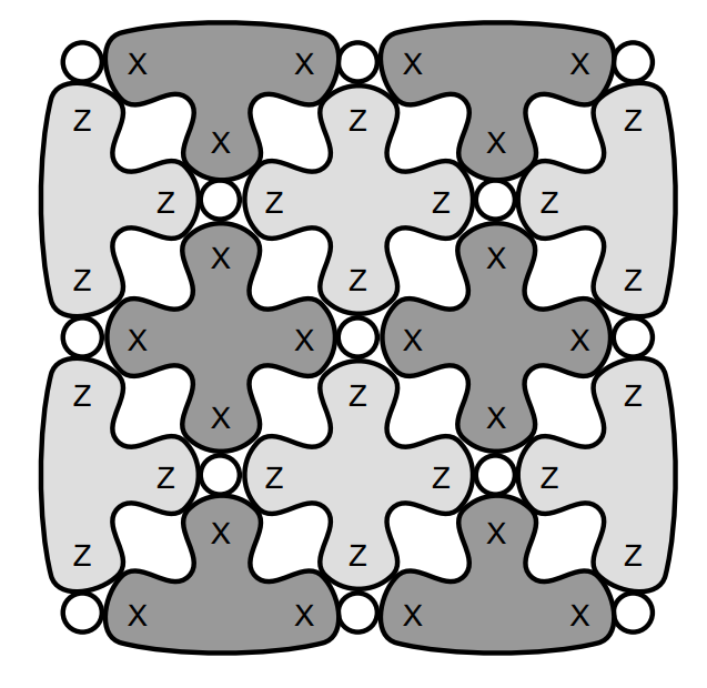
A distance \(d=3\) surface code. Circles represent qubits and bubbles represent operators, called stabilizers, used to detect errors. The stabilizers are tensor products of Pauli-\(X\) or Pauli-\(Z\) operators and each is associated with its own ancilla qubit. The combined system encodes one logical qubit and can correct any combination of \(\lfloor (d-1)/2 \rfloor\) errors. 19

In the measurement-based picture, quantum error correction requires cluster states that are at least 3-dimensional 3, contrary to the 2-dimensional cluster states required for universal quantum computation discussed in the previous section. The error correcting code that you want to implement dictates the structure of the cluster state. The cluster state that is associated with the surface code is known as the RHG lattice, named after its architects Raussendorf, Harrington, and Goyal. We can visualize this cluster state with FlamingPy.

from flamingpy.codes import SurfaceCode

code_distance = 3
RHG = SurfaceCode(code_distance)

fig, _ = RHG.draw(backend="matplotlib", showbackground=True)
plt.show()

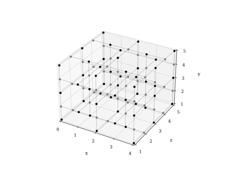
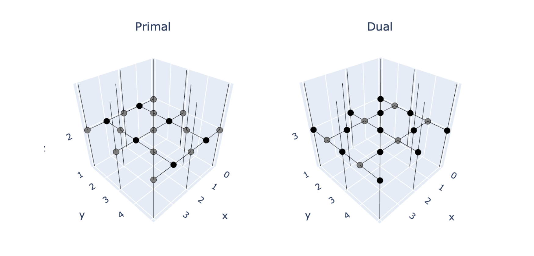
For the sake of intuition, you can think of the graph shown above as having two spatial dimensions (\(x\) and \(y\)) and one temporal dimension (\(z\)). The cluster state alternates between primal and dual sheets, shown below in more detail. In principle, any quantum error correction stabilizer code can be foliated into a graph state for measurement-based QEC 15, 22. However, the foliations are particularly nice for CSS codes, named after Calderbank, Shor, and Steane. CSS codes have stabilizers that exclusively contain \(X\)-stabilizers or \(Z\)-stabilizers, and include the surface code and colour code families. For these CSS codes, you can roughly view the primal and dual sheets as measuring the \(Z\)-stabilizers and \(X\)-stabilizers, respectively. We encourage you to have another look at the figure with the distance-3 surface code and try to link it with the dual and primal sheets shown here!

The computation and error correction are again performed with single-qubit measurements, as illustrated below. At each timestep, we measure all the qubits on one sheet of the lattice. The binary outcomes of these measurements determine the measurement bases for future measurements, and the last sheet of the lattice contains the encoded result of the computation which can be read out by yet another measurement.

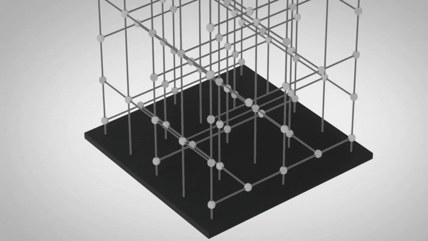
Performing an error corrected computation with measurements using the RHG lattice. 3

Conclusion

We have learned that a one-way quantum computer capable of cluster state entanglement together with adaptive arbitrary single-qubit measurements allows for universal quantum computation. The MBQC framework is a powerful quantum computing approach, particularly useful in platforms that allow for many expendable flying qubits and easy physical entangling gates. It circumvents the need for applying in-line entangling gates that are often the most noisy operations in gate-based quantum computers with trapped-ions or superconducting circuits. Instead, the required entanglement is created off-line which is often simpler to implement. Furthermore, it’s advantageous for photonics because the depth of the optical circuit can remain constant. This means that it does not grow with the depth of the logical circuit, preventing intolerable losses.

In this demo, we assumed that the system is capable of performing arbitrary single-qubit measurements. This is not a strict requirement, as one can acquire the same capabilities by sprinkling magic states into the cluster state. A discussion of this topic is beyond the scope of this tutorial, but a good place to start is this paper 16.

Xanadu’s approach toward a universal quantum computer involves continuous-variable cluster states 9. If you would like to learn more about the architecture, you can read our blueprint papers 3 and 4. We also highly recommend watching this video outlining the main ideas!

References

1(1,2,3,4)

Robert Raussendorf and Hans J. Briegel (2001) A One-Way Quantum Computer, Phys. Rev. Lett. 86, 5188.

2(1,2)

Swapnil Nitin Shah (2021) Realizations of Measurement Based Quantum Computing, arXiv.

3(1,2,3)

J. Eli Bourassa, Rafael N. Alexander, Michael Vasmer, Ashlesha Patil, Ilan Tzitrin, Takaya Matsuura, Daiqin Su, Ben Q. Baragiola, Saikat Guha, Guillaume Dauphinais, Krishna K. Sabapathy, Nicolas C. Menicucci, and Ish Dhand (2021) Blueprint for a Scalable Photonic Fault-Tolerant Quantum Computer, Quantum 5, 392.

4(1,2,3)

Ilan Tzitrin, Takaya Matsuura, Rafael N. Alexander, Guillaume Dauphinais, J. Eli Bourassa, Krishna K. Sabapathy, Nicolas C. Menicucci, and Ish Dhand (2021) Fault-Tolerant Quantum Computation with Static Linear Optics, PRX Quantum, Vol. 2, No. 4.

5

Peter W. Shor (1995) Scheme for reducing decoherence in quantum computer memory, Physical Review A, Vol. 52, Iss. 4.

6

Daniel Herr, Alexandru Paler, Simon J. Devitt and Franco Nori (2018) Lattice Surgery on the Raussendorf Lattice, IOP Publishing 3, 3.

7

Austin G. Fowler, Matteo Mariantoni, John M. Martinis, Andrew N. Cleland (2012) Surface codes: Towards practical large-scale quantum computation, arXiv.

8

Google Quantum AI (2022) Suppressing quantum errors by scaling a surface code logical qubit, arXiv.

9

Nicolas C. Menicucci, Peter van Loock, Mile Gu, Christian Weedbrook, Timothy C. Ralph, and Michael A. Nielsen (2006) Universal Quantum Computation with Continuous-Variable Cluster States, arXiv.

10

David P. DiVincenzo. (2000) The Physical Implementation of Quantum Computation, arXiv.

11

A. Furusawa, J. L. Sørensen, S. L. Braunstein, C. A. Fuchs,H. J. Kimble, E. S. Polzik. (1998) Unconditional Quantum Teleportation, Science Vol 282, Issue 5389.

12

M. A. Nielsen, E. Knill & R. Laflamme. (1998) Complete quantum teleportation using nuclear magnetic resonance, Nature volume 396, 52–55.

13

S. L. N. Hermans, M. Pompili, H. K. C. Beukers, S. Baier, J. Borregaard & R. Hanson. (2022) Qubit teleportation between non-neighbouring nodes in a quantum network, Nature 605, 663–668.

14

M. Riebe, H. Häffner, C. F. Roos, W. Hänsel, J. Benhelm, G. P. T. Lancaster, T. W. Körber, C. Becher, F. Schmidt-Kaler, D. F. V. James & R. Blatt. (2002) Deterministic quantum teleportation with atoms, Nature 429, 734-737.

15

A. Bolt, G. Duclos-Cianci, D. Poulin, T. M. Stace. (2016) Foliated Quantum Codes, arXiv.

16

Sergey Bravyi and Alexei Kitaev. (2004) Universal quantum computation with ideal Clifford gates and noisy ancillas, arXiv.

17

M. Hein, J. Eisert and H.J. Briegel. (2003) Multi-party entanglement in graph states, arXiv.

18

Jeremy L. O’Brien. (2007) Optical quantum computing, Science Vol. 318, Issue 5856, 1567-1570.

19(1,2)

Austin G. Fowler. (2013) Polyestimate: instantaneous open source surface code analysis, arXiv.

20

M. Hein, W. Dür, J. Eisert, R. Raussendorf, M. Van den Nest, H.J. Briegel. (2006) Entanglement in Graph States and its Applications, arXiv.

21

Hans J. Briegel and Robert Raussendorf (2001) Persistent Entanglement in Arrays of Interacting Particles, Phys. Rev. Lett. 86, 910.

22

Benjamin J. Brown, Sam Roberts. (2018) Universal fault-tolerant measurement-based quantum computation, arXiv.

About the authors

Joost Bus

I am a MSc student in Quantum Engineering at ETH Zürich who likes to explore how to wield quantum physics for technology. This summer, I am working with the architecture team on FlamingPy as a Xanadu resident.

Radoica Draskic

I am a trained theoretical physicist and a wannabe computer scientist. I am currently working as a summer resident at Xanadu.

demos/tutorial_mbqc

 

Download Python script

 

Download Notebook

 

View on GitHub