Note
Click here to download the full example code
Introduction to the ZX-calculus
Author: Romain Moyard. Posted: 6 June, 2023.
The ZX-calculus is a graphical language for reasoning about quantum computations and circuits. Introduced by Coecke and Duncan 1, it can represent any linear map, and can be considered a diagrammatically complete generalization of the usual circuit representation. The ZX-calculus is based on category theory, an approach to mathematics which studies objects in terms of their relations rather than in isolation. Thus, the ZX-calculus provides a rigorous way to understand the structure underlying quantum problems, using the link between quantum operations rather than the quantum operations themselves.
After this tutorial you will understand how to represent quantum teleportation and simplify it in the ZX-calculus!
In this tutorial, we first give an overview of the building blocks of the ZX-calculus, called ZX-diagrams, and the rules for transforming them, called rewriting rules. We also show how the ZX-calculus can be extended to ZXH calculus. The ZX-calculus is also promising for quantum machine learning, thus we present how the parameter-shift rule can be derived using ZX-diagrams. We will then jump to the coding part of the tutorial and show how PennyLane is integrated with PyZX 2, a Python library for ZX-calculus, and how you can transform your circuit to a ZX-diagram. We then apply what we’ve learned in order to optimize the number of T-gates of a known benchmark circuit. We also show that simplifying a ZX-diagram does not always end up with a diagram-like graph, and that circuit extraction is a main pain point of the ZX framework. This tutorial will give a broad overview of what ZX-calculus can offer when you want to analyze quantum problems.
ZX-diagrams
This introduction follows the works of the East et al. 3 and van de Wetering 4. Our goal is to introduce a complete language for quantum information, for which we need two elements: ZX-diagrams and their rewriting rules. We start by introducing ZX-diagrams, a graphical depiction of a tensor network representing an arbitrary linear map. Later, we will introduce ZX rewriting rules, which together with diagrams defines the ZX-calculus. We follow the scalar convention of East et al. 3 (it is more suitable to the multi-H box situations, see the ZXH section).
A ZX-diagram is an undirected multi-graph; you can move vertices without affecting the underlying linear map. The vertices are called Z- and X-spiders, which represent two kinds of linear maps. The edges are called wires, and represent the dimensions on which the linear maps are acting. Therefore, the edges represent qubits in quantum computing. The diagram’s wires on the left and right are called inputs and outputs, respectively.
The first building block of the ZX-diagram is the Z-spider. In most of the literature, it is depicted as a green vertex. The Z-spider takes a real phase \(\alpha \in \mathbb{R}\) and represents the following linear map (it accepts any number of inputs and outputs, and the number of inputs does not need to match the number of outputs):
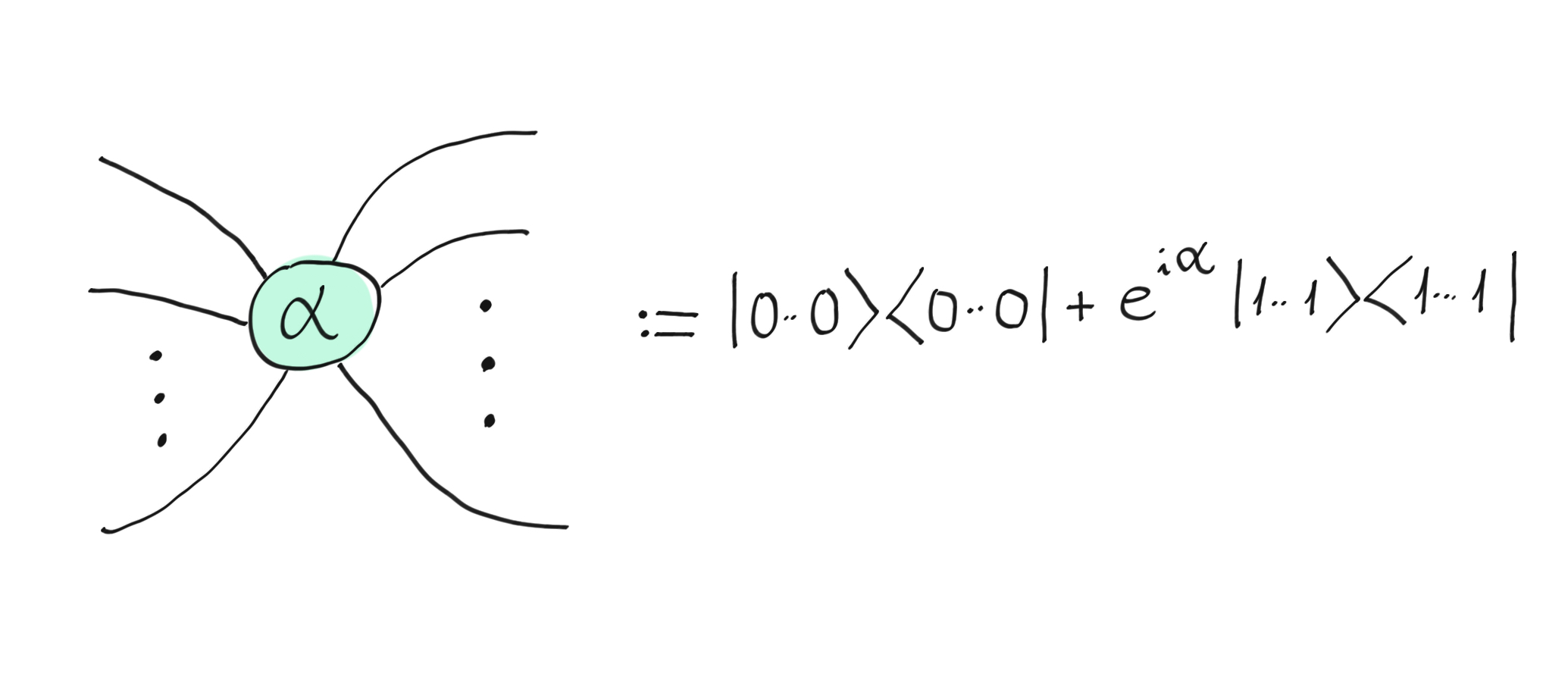
The Z-spider.
It is easy to see that the usual Z-gate can be represented with a single-wire Z-gate:
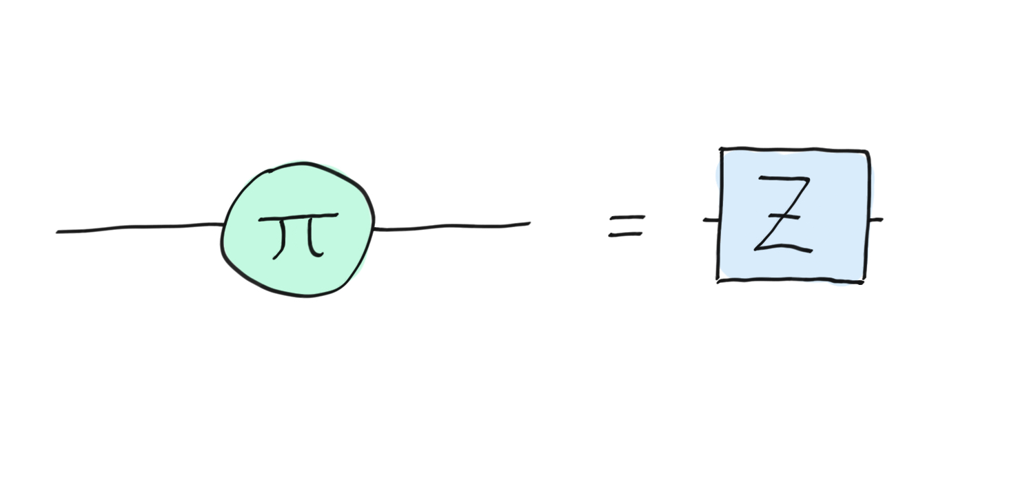
The Z-gate.
As you’ve probably already guessed, the second building block of the ZX-diagram is the X-spider. It is usually depicted as a red vertex. The X-spider also takes a real phase \(\alpha \in \mathbb{R}\) and it represents the following linear map (it accepts any number of inputs and outputs):
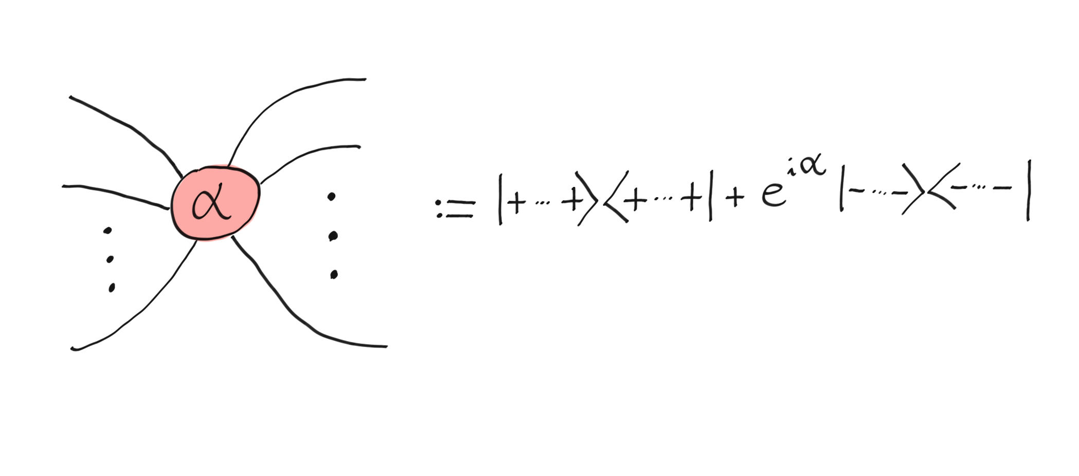
The X-spider.
It is easy to see that the usual X-gate can be represented with a single-wire X-spider:
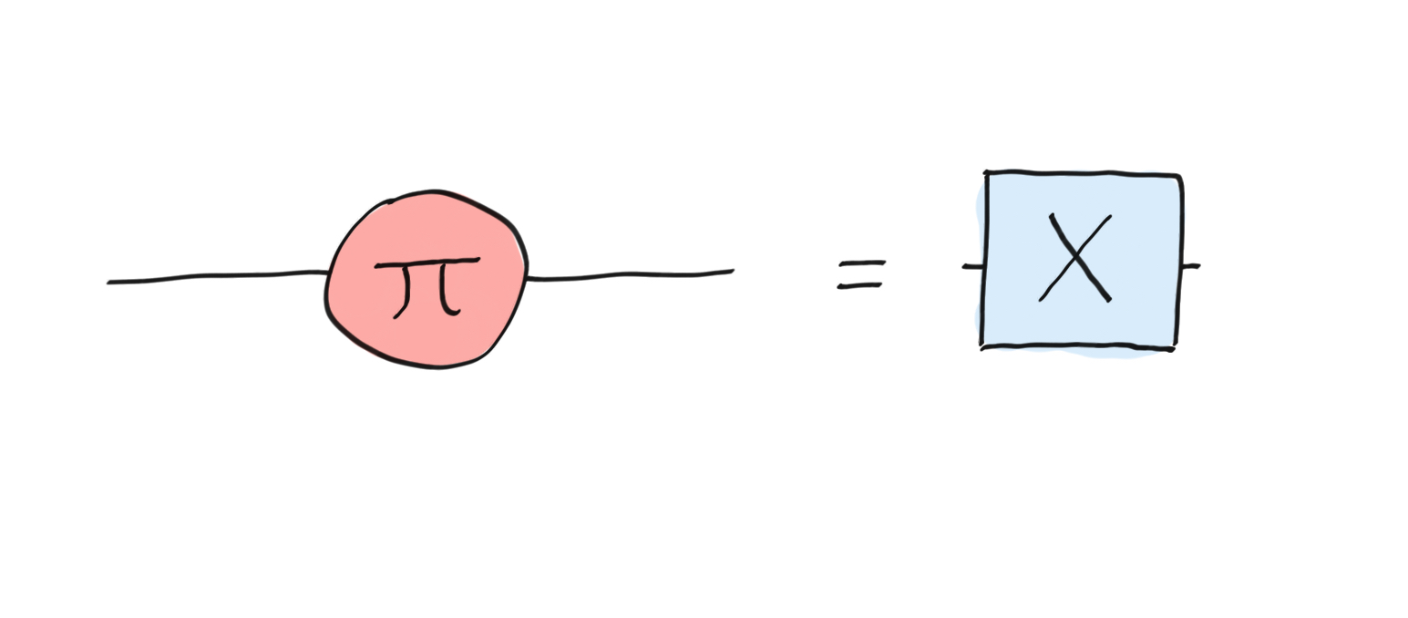
The X-gate.
From ordinary quantum theory, we know that the Hadamard gate can be decomposed into X and Z rotations, and can therefore be represented in ZX-calculus. In order to make the diagram easier to read, we introduce the Hadamard gate as a yellow box:
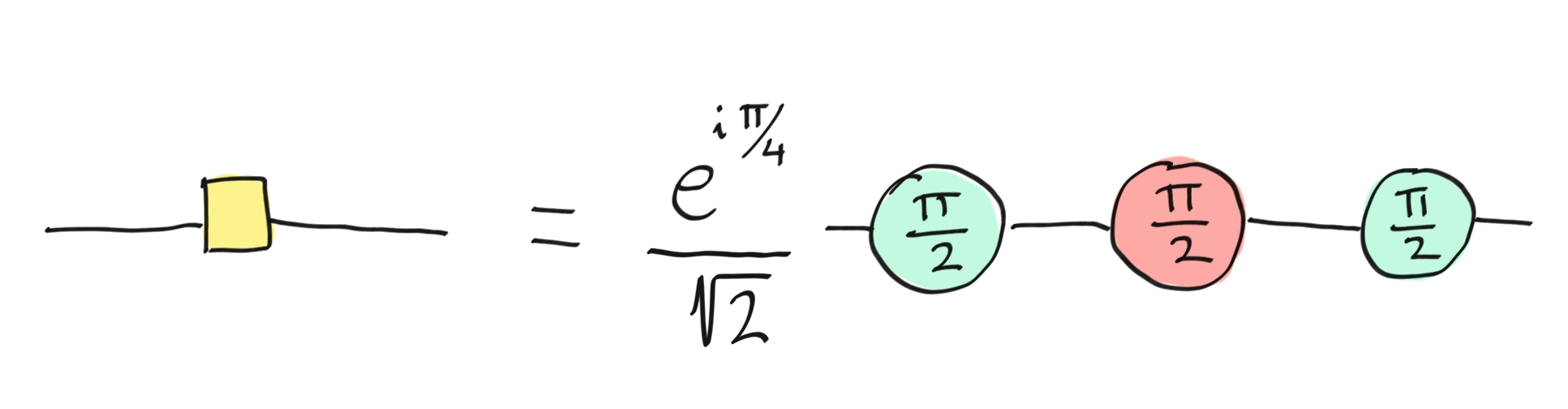
The Hadamard gate as a yellow box and its ZX decomposition.
This yellow box is also often represented as a blue edge in order to further simplify the display of the diagram. Below, we will discuss a generalization of the yellow box to a third spider, forming the ZXH-calculus. It is important to note that the yellow box is by itself a rewrite rule for the decomposition of the Hadamard gate. The yellow box allows us to write the relationship between the X- and Z-spider as follows.
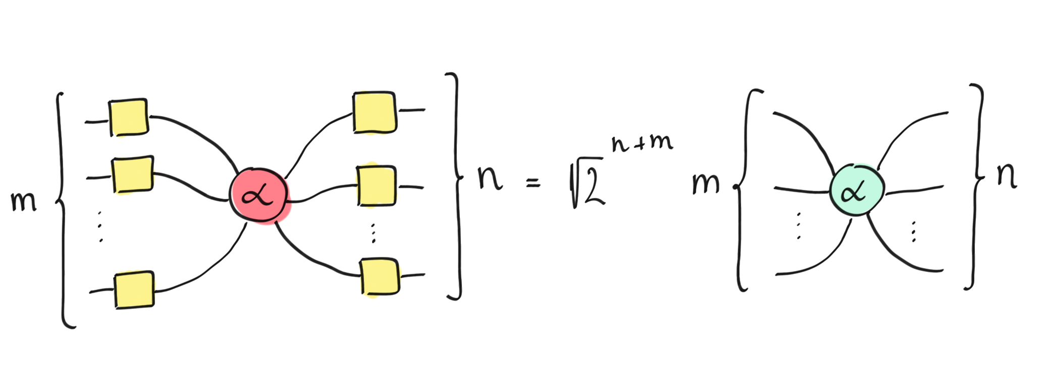
How to transform an X-spider to a Z-spider with the Hadamard gate.
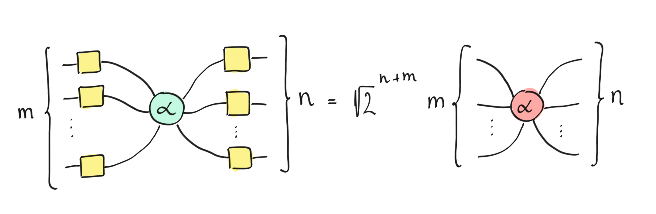
How to transform an Z-spider to a X-spider with the Hadamard gate.
A special case of the Z- and X-spiders are diagrams with no inputs (or outputs). They are used to represent states that are unnormalized. If a spider has no inputs and outputs, it simply represents a complex scalar. You can find the usual representation of quantum states below:
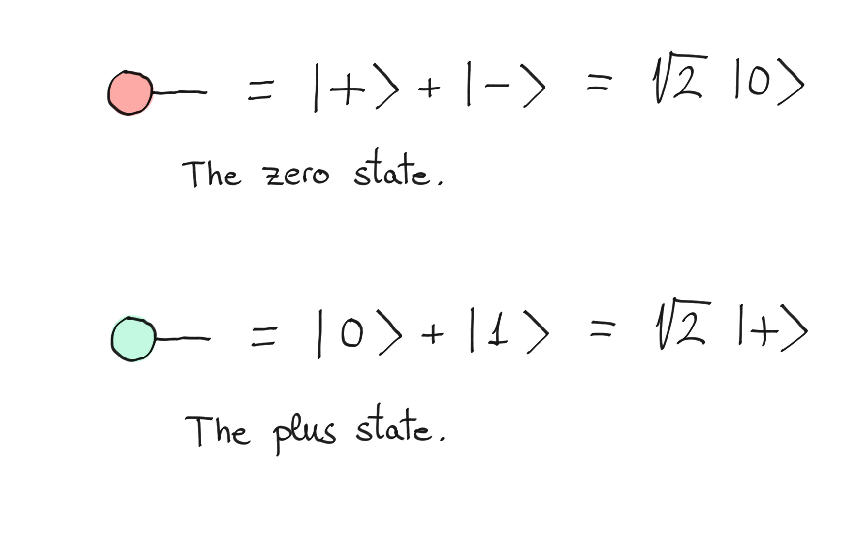
The zero state and plus state as a ZX-diagram.
Similarly, you get the \(\vert 1\rangle\) state and \(\vert -\rangle\) state by replacing the zero phase with \(\pi\).
The phases are \(2\pi\) periodic, and when a phase is equal to \(0\) we omit the zero symbol from the spider. A simple green vertex is a Z-spider with zero phase and a simple red vertex is an X-spider with zero phase.
Now that we have these two basic building blocks, we can start composing them and stacking them on top of each other. Composition consists of joining the outputs of a diagram to the inputs of another diagram. Stacking two ZX-diagrams on top of each other represents the tensor product of the corresponding tensors.
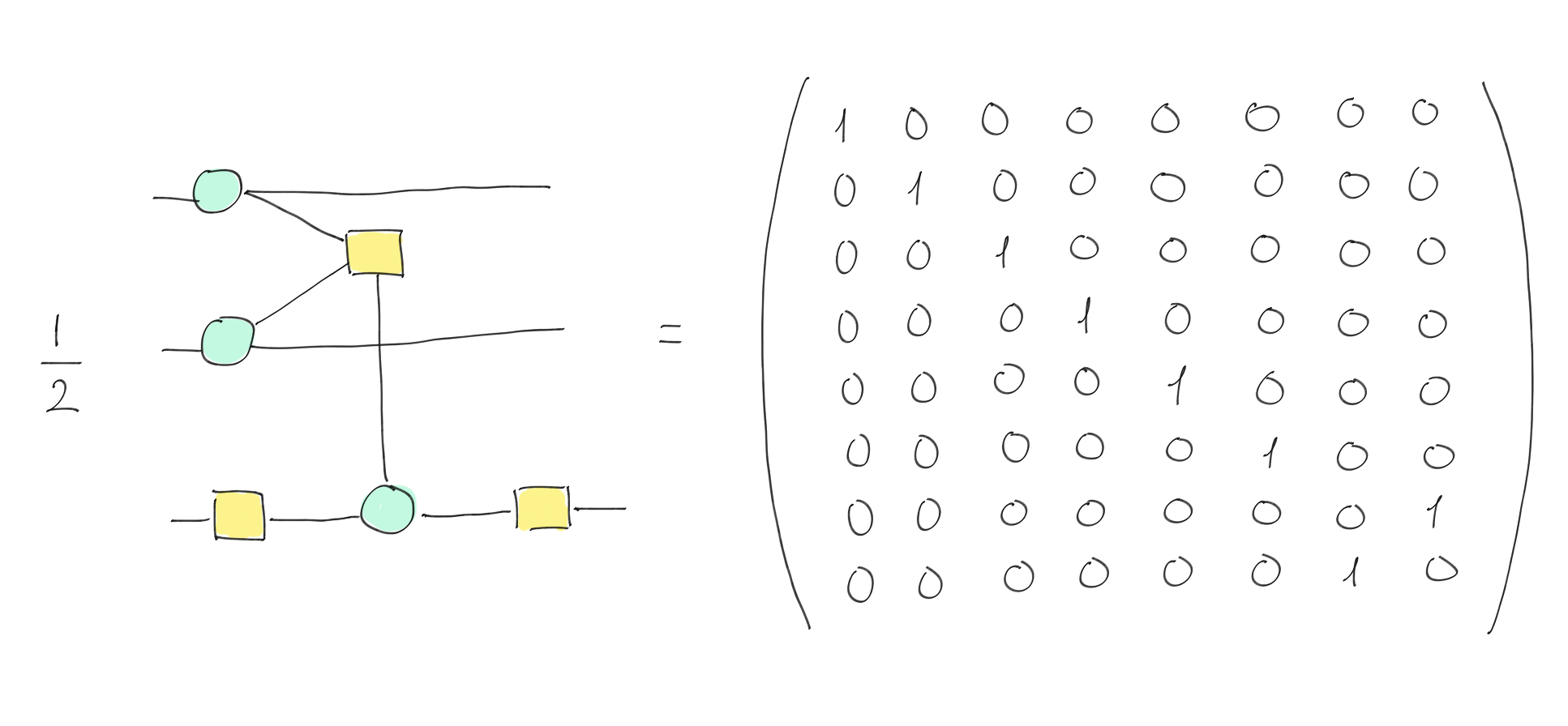
We illustrate the rules of stacking and composition by building an equivalent CNOT gate (up to a global phase). We start by stacking a single wire with a phaseless Z-spider with one input wire and two output wires. We show the ZX-diagram and corresponding matrix below:
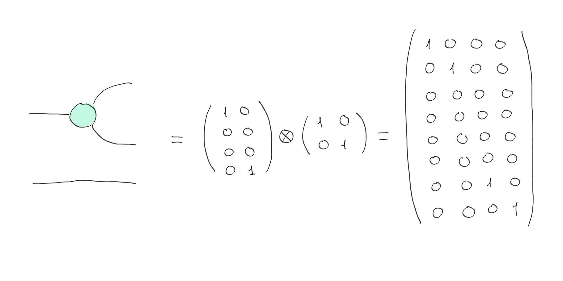
Phaseless Z-spider with one input wire and two output wires (see the definition of the Z-spider) stacked with a single wire.
Next, we stack a single wire with a phaseless X-spider with two input wires and single output wire. Again, we provide the matrix:
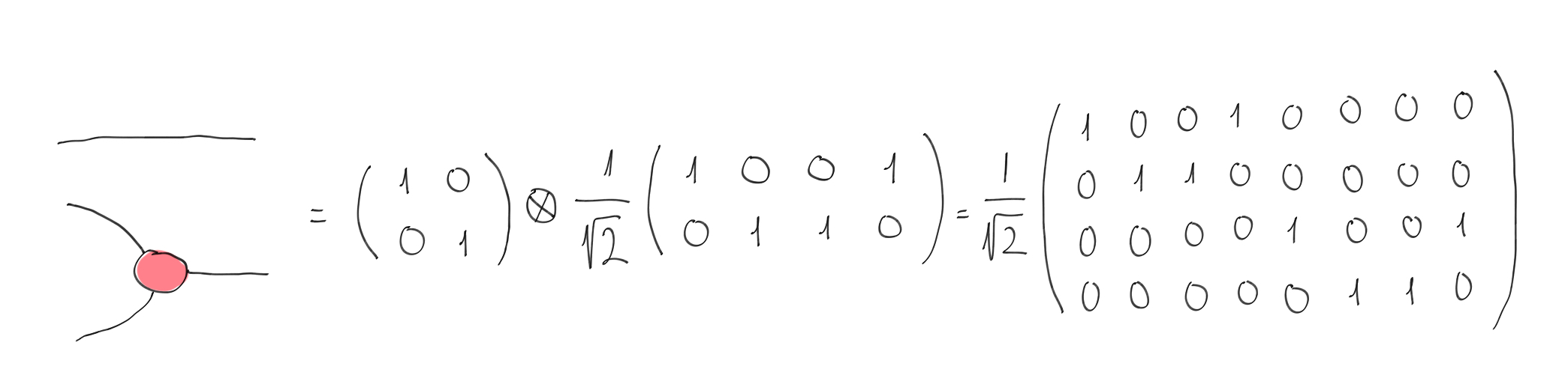
Single wire stacked with a phaseless X-spider with two inputs wires and one output wire.
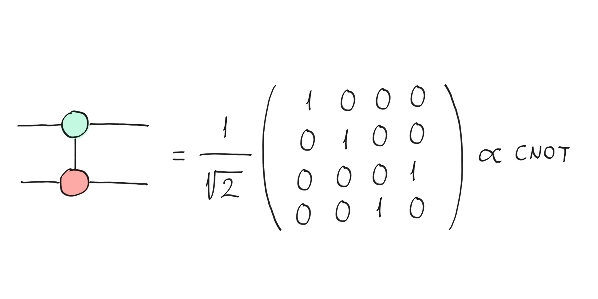
Finally, we compose the two diagrams, meaning that we join the two outputs of the first diagram with the two inputs of the second diagram. By doing this we obtain a CNOT gate — you can convince yourself by doing the matrix multiplication between the two diagrams.
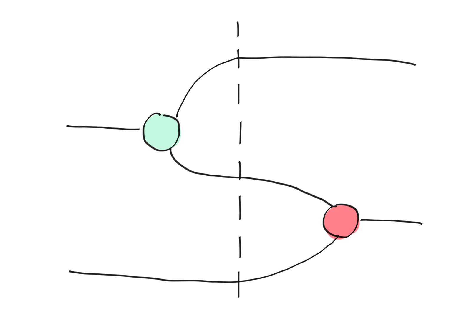
The composition of the two diagrams is a CNOT gate.
We’ve already mentioned that a ZX-diagram is an undirected multi-graph; the position of the vertices does not matter, nor does the trajectory of the wires. We can move vertices around, bend and unbend, and cross and uncross wires as long as the connectivity and the order of the inputs and outputs is maintained. In particular, bending a line so that it changes direction from left to right, or vice-versa, is not allowed. None of these deformations affect the underlying linear map, meaning that ZX-diagrams have all sorts of topological symmetries. For instance, the two diagrams below both represent the CNOT gate:
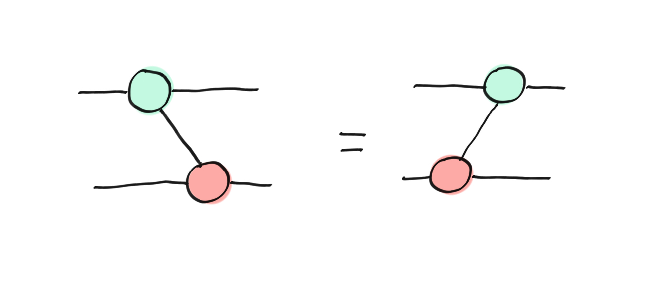
Both diagrams represent the same CNOT gate.
This means that we can draw a vertical line without ambiguity, which is the usual way of representing the CNOT gate:
Usual representation of the CNOT gate as a ZX-diagram.
We’ve just shown that we can express any Z rotation and X rotation with Z- and X-spiders. Therefore, it is sufficient to create any one-qubit rotation on the Bloch sphere. By composing and stacking, we can also create the CNOT gate. Therefore, we have a universal gate set! We can also create the \(0\) state and \(+\) state on any number of qubits. Therefore, we can represent any quantum state. Normalization might be needed (e.g., for the CNOT gate) and we perform this by adding complex scalar vertices.
It turns out that the ability to represent an arbitrary state implies the ability to represent an arbitrary linear map. Using a mathematical result called the Choi-Jamiolkowski isomorphism 4, for any linear map \(L\) from \(n\) to \(m\) wires, we can bend the incoming wires to the right and find an equivalent state on \(n + m\) wires. Thus, any linear map is equivalent to some state, and since we can create any state, we can create any map! This shows that ZX-diagrams are a universal tool for reasoning about linear maps. But this doesn’t mean the representation is simple!
ZX-calculus: rewriting rules
ZX-diagrams coupled with rewriting rules form the ZX-calculus. Previously, we presented the rules for composing and stacking diagrams and talked about the topological symmetries corresponding to deformations. In this section, we provide rewriting rules that can be used to simplify diagrams without changing the underlying linear map. This can be very useful for quantum circuit optimization and for showing that some computations have a very simple form in the ZX framework (e.g., teleportation).
In the following rules, the colours are interchangeable.
Since the X-gate and Z-gate do not commute, non-phaseless vertices of different color do not commute.
The fuse rule applies when two spiders of the same type are connected by one or more wires. We can fuse spiders by simply adding the two spiders’ phases and removing the connecting wires.
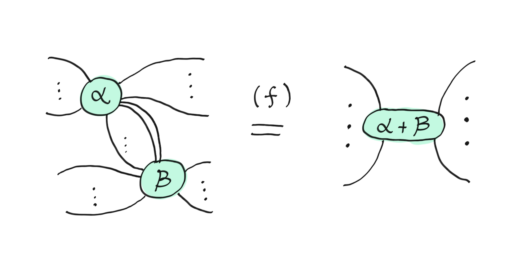
The (f)use rule.
The \(\pi\) -copy rule describes how to pull an X-gate through a Z-spider (or a Z-gate through an X-spider). Since X and Z anticommute, pulling the X-gate through a Z-spider introduces a minus sign into the Z phase.
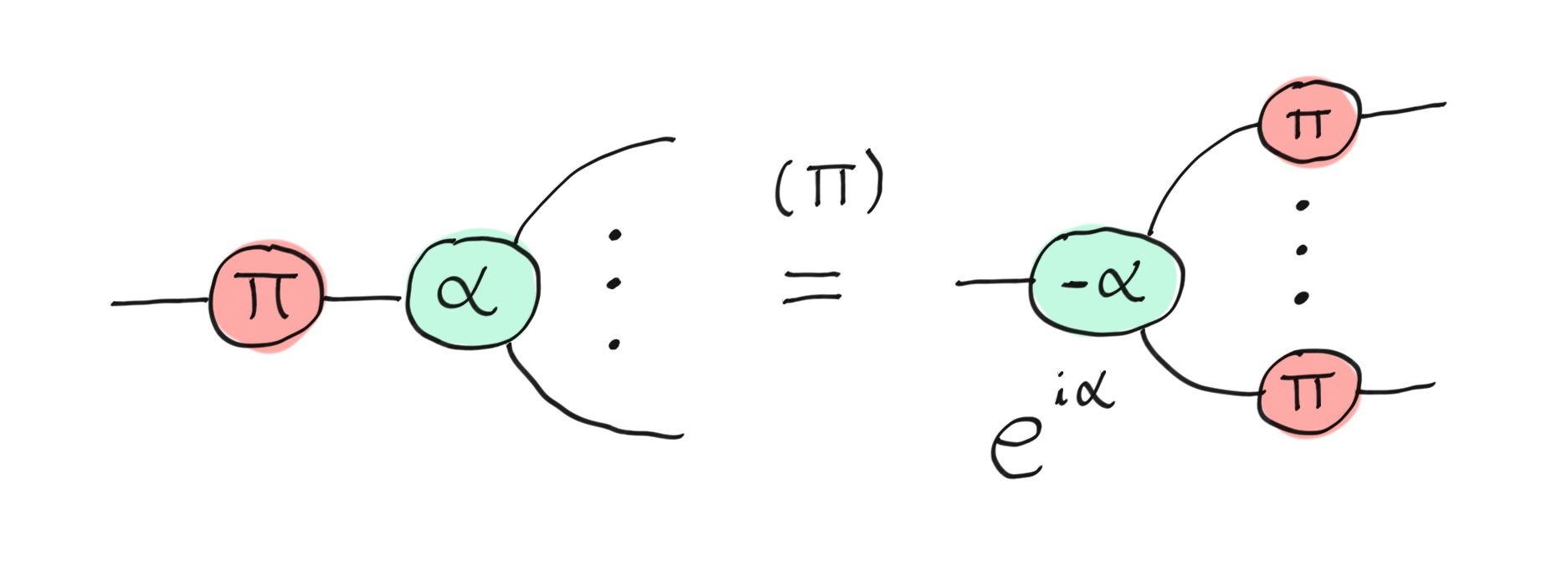
The (\(\pi\))-copy rule.
The state-copy rule captures how simple one-qubit states interact with a spider of the opposite colour. It is only valid for states that are multiples of \(\pi\) (therefore \(a\) is an integer), so we have computational basis states (in the X or Z basis). Basically, if you pull a basis state through a spider of the opposite color, it copies it onto each outgoing wire.
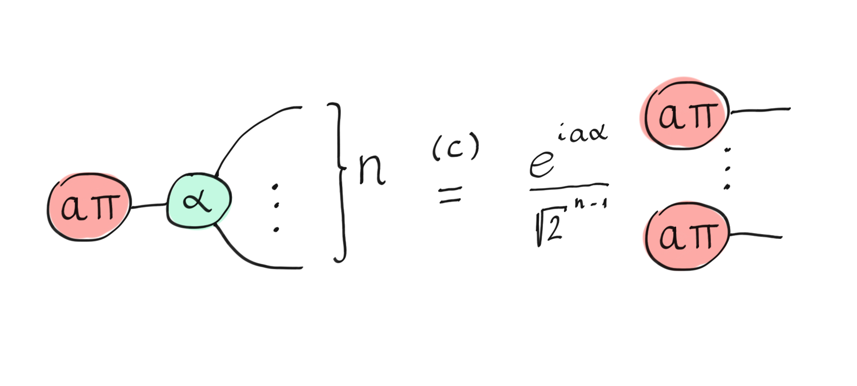
The state (c)opy rule, where \(a\) is an integer.
The identity rule states that phaseless spiders with one input and one output are equivalent to the identity and can therefore be removed. This is similar to the rule that Z and X rotation gates, which are phaseless, are equivalent to the identity. This rule provides a way to get rid of self-loops.
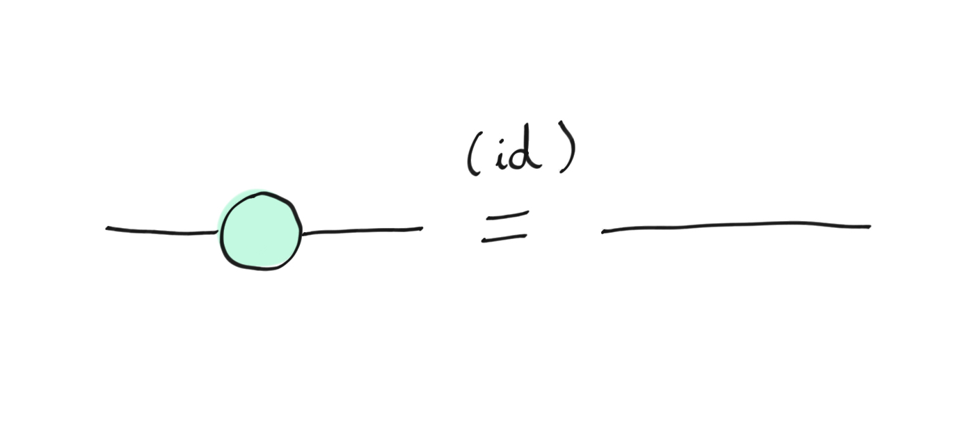
The (id)entity removal rule.
A bialgebra is a mathematical structure with a product (combining two wires into one) and a coproduct ( splitting a wire into two wires) where, roughly speaking, we can pull a product through a coproduct at the cost of doubling. This is similar to the relation enjoyed by the XOR algebra and the COPY coalgebra. This rule is not straightforward to verify and details can be found in 4 .
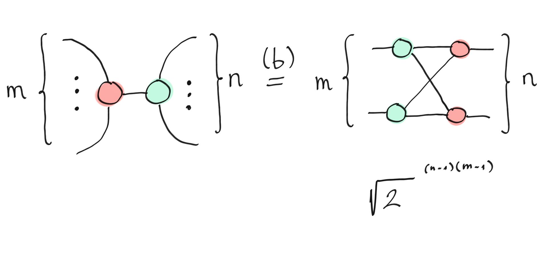
The (b)ialgebra rule.
The Hopf rule is a bit like the bialgebra rule, telling us what happens when we try to pull a coproduct through a product. Instead of doubling, however, they decouple, leaving us with an unconnected projector and a state. Again, this relation is satisfied by XOR and COPY, and the corresponding algebraic structure is called a Hopf algebra. This turns out to follow from the bialgebra and the state-copy rule 4, but it’s useful to record it as a separate rule.
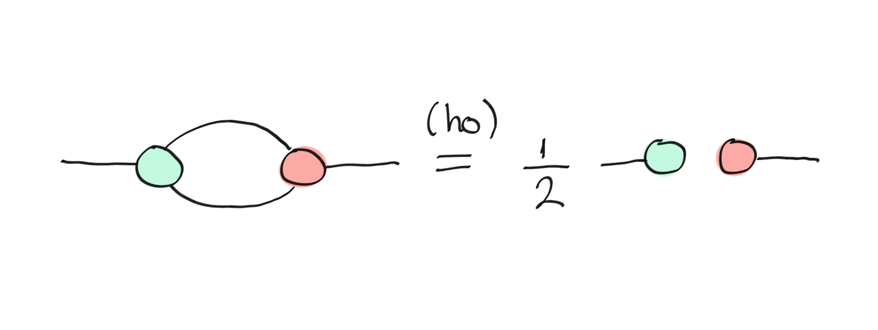
The (ho)pf rule.
Teleportation
Now that we have all the necessary tools, let’s see how to describe teleportation as a ZX-diagram and simplify it with our rewriting rules. The results are surprisingly elegant! We follow the explanation from 4. You can find an introduction to teleportation in the MBQC demo.
Teleportation is a protocol for transferring quantum information (a state) from Alice (the sender) to Bob (the receiver). To perform this, Alice and Bob first need to share a maximally entangled state. The protocol for Alice to send her quantum state to Bob is as follows:
Alice applies the CNOT gate followed by the Hadamard gate.
Alice measures the two qubits that she has.
Alice sends the two measurement results to Bob.
Given the results, Bob conditionally applies the Z- and X-gate to his qubit.
Bob ends up with the same state as Alice previously had. Teleportation is complete!
In the ordinary quantum circuit notation, we can summarize the procedure as follows:
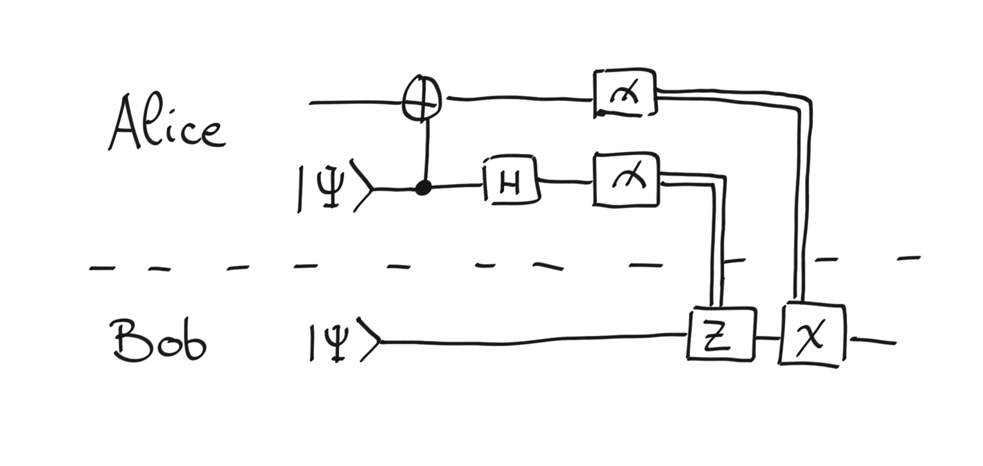
The teleportation circuit.
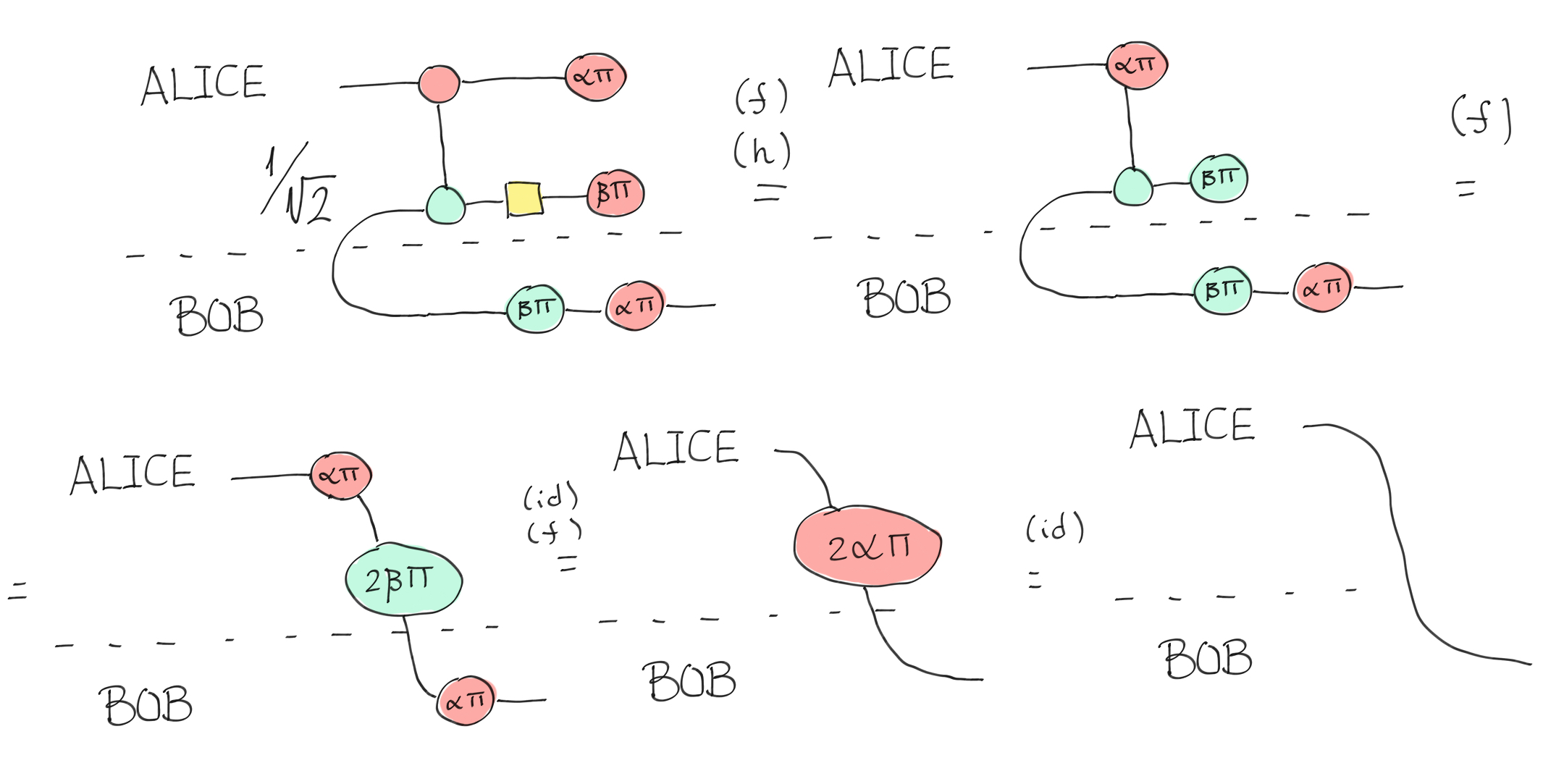
Let us convert this quantum circuit into a ZX-diagram. The measurements are represented by the state X-spider parameterized with boolean parameters \(\alpha\) and \(\beta\). The cup represents the maximally entangled state shared between Alice and Bob. As you might expect from earlier comments about bending wires, their shared state is Choi-Jamiolkowski-equivalent to the identity linear map.
Let’s simplify the diagram by applying some rewriting rules. The first step is to fuse the \(a\) state with the X-spider of the CNOT. We also merge the Hadamard gate with the \(\beta\) state, because together it represents a Z-spider. Then we can fuse the three Z-spiders by simply adding their phases. After that, we see that the Z-spider phase vanishes (modulo \(2\pi\)) and can therefore be simplified using the identity rule. Then we can fuse the two X-spiders by adding their phases. We notice that the phase again vanishes modulo \(2\pi\) and we can get rid of the last X-spider. Teleportation is a simple wire connecting Alice and Bob!
The ZXH-calculus
The universality of the ZX-calculus does not guarantee the existence of a simple representation, even for simple linear maps. For example, the Toffoli gate (the quantum AND gate) requires around 25 spiders (Z and X)! We previously introduced the Hadamard gate as a yellow box, which motivates the introduction of a new generator: the multi-leg H-box, defined as follows:
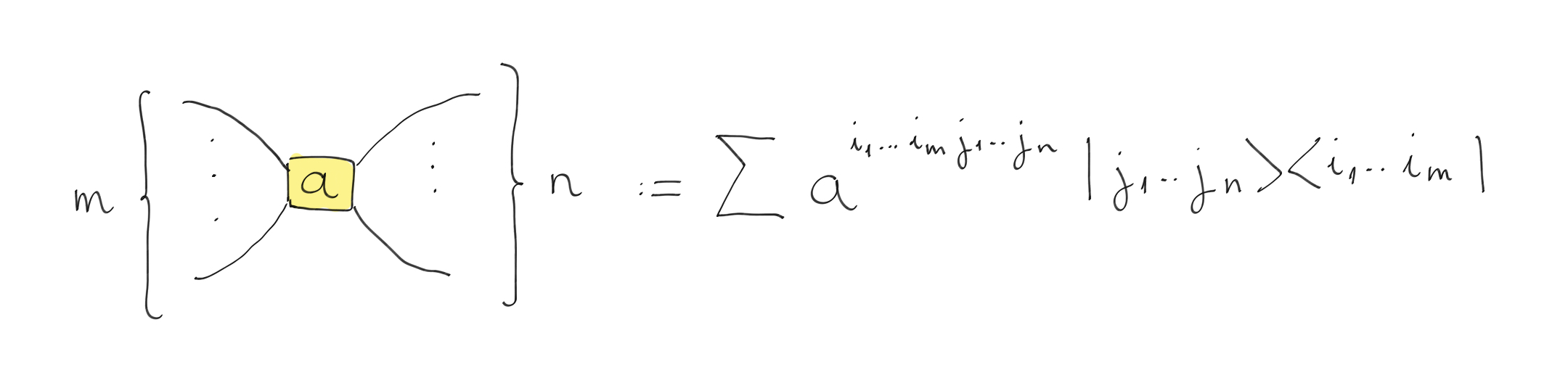
The H-box, a third generator.
The parameter \(a\) can be any complex number, and the sum is over all \(i_1, ... , i_m, j_1, ... , j_n \in \{0, 1\}\). Therefore, an H-box represents a matrix where its entries are equal to \(1\) except for the bottom right element, which is \(a\). This will allow us to concisely express the Toffoli gate, as we will see shortly.
An H-box with one input wire and one output wire, with \(a=-1\), is a Hadamard gate up to global phase. Thus, we omit the parameter when it is equal to \(-1\). The Hadamard gate is sometimes represented by a blue edge rather than a box.
Thanks to the introduction of the multi-leg H-box, the Toffoli gate can be represented with three Z-spiders and three H-boxes — two simple Hadamard gates and one three-ary H-box — as shown below:
Toffoli
The addition of the multi-leg H-box together with an additional set of rewriting rules forms the ZXH-calculus. You can find more details and the rewriting rules in the literature 3.
Let’s show that this ZXH-diagram is indeed a Toffoli-gate. This operation is defined by conditionally applying an X-gate on the target wire, it means that only the state \(|110\rangle\) and \(|111\rangle\) will not map to themselves (\(|110\rangle\) to \(|111\rangle\) and \(|111\rangle\) to \(|110\rangle\)). We will show that if one provides the state \(|11\rangle\) on the two first wires, it results to a bit flip on the third wire (X-gate). For that purpose, we need to add a new rewriting rule that is part of the ZXH-calculus: the absorb rule.
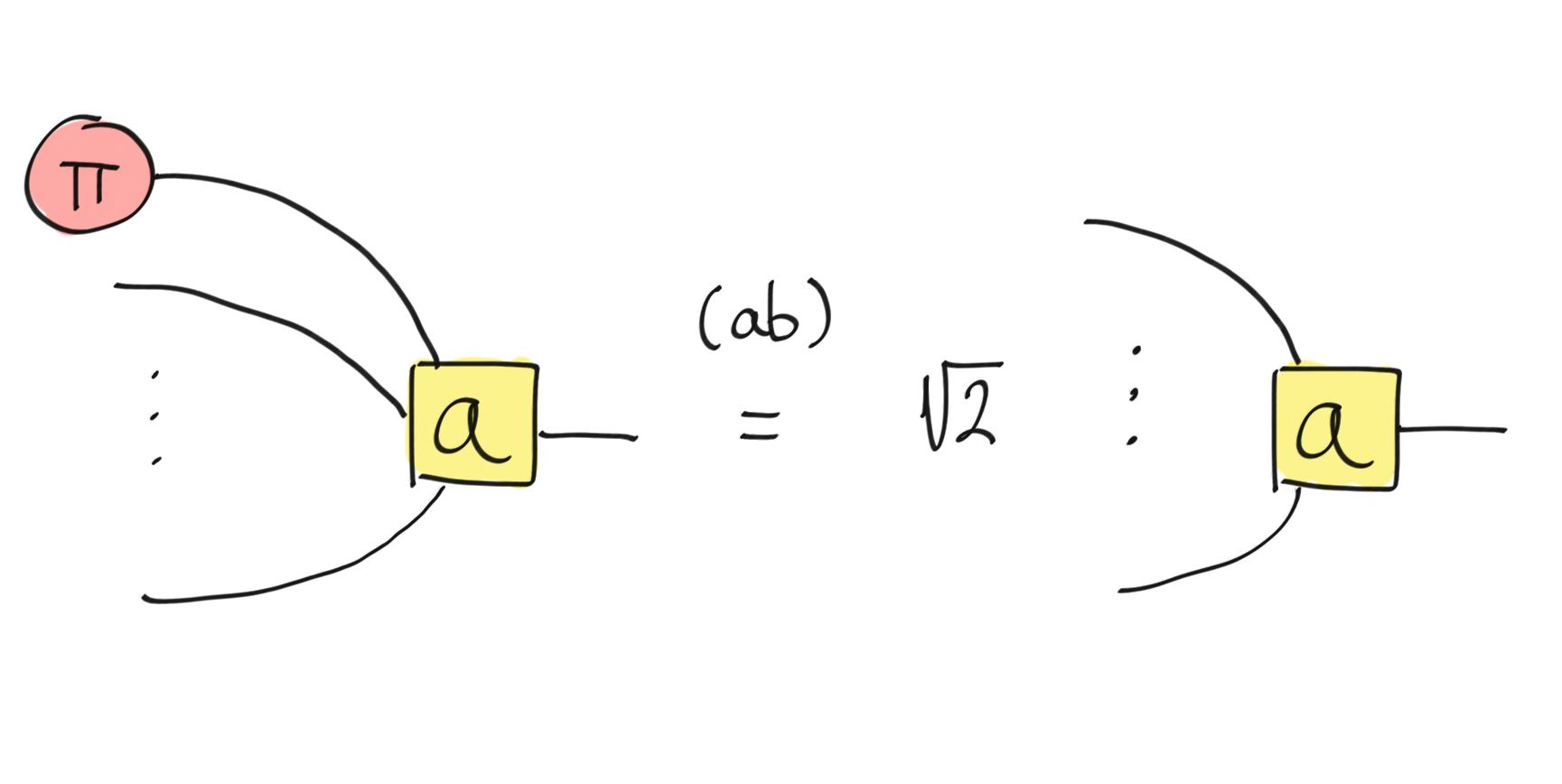
The (ab)sorb rule.
We start by applying our Toffoli diagram on a \(|11\rangle\) state, which corresponds to two X-spiders with a phase of \(\pi\) stacked with our diagram. We apply the copy rule on the two groups of X-spiders and Z-spiders on the wires 0 and 1. After that we can apply the newly introduced absorb rule on one of the X-spiders connected to the H-Box. Then we recognize the Fourier relation and can replace the X-spider and H-Box by a Z-spider. Then it is easy to apply the fuse rule on the two Z-spiders. Again, we recognize the Fourier relation and obtain a single X-spider on the target wire. We just proved that by providing the \(|11\rangle\) state on the two control wires, it always applies an X-spider on the target. It means that we have a bit flip on the target.
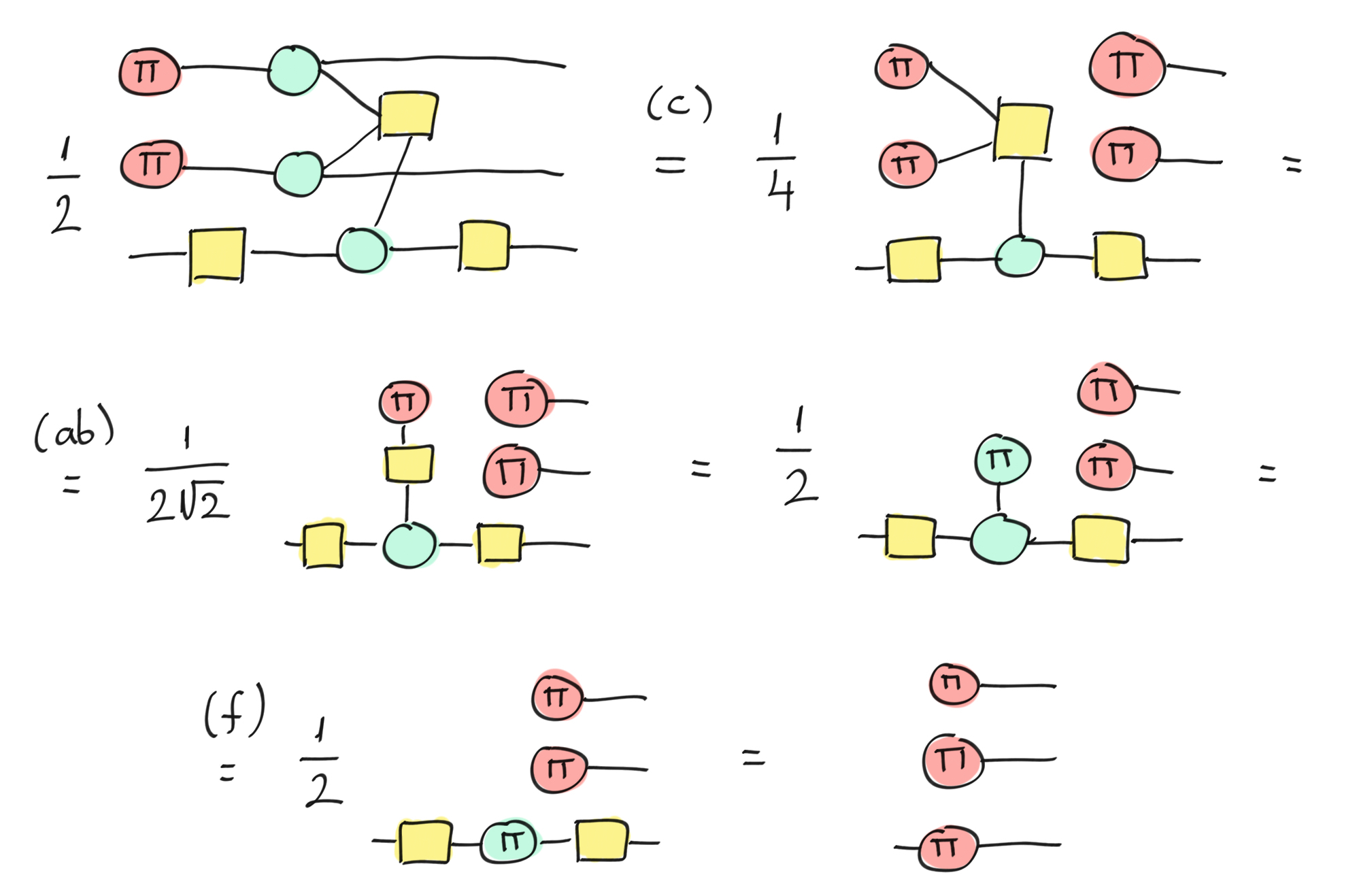
Toffoli-diagram applied on the \(|11\rangle\) state.
If you do the same procedure with the others states on the two controls (\(|00\rangle\), \(|11\rangle\), \(|10\rangle\), \(|01\rangle\)) with slightly different rules (the explosion rule), you will always end up with an empty target and identical states for the controls. We then have proved that our ZXH-diagram is indeed the Toffoli gate!
The ZX-calculus for quantum machine learning
We now move away from the standard use of the ZX-calculus in order to show its utility for calculus and, more specifically, for quantum derivatives (the parameter-shift rule). What follows is not implemented in PennyLane or PyZX. By adding derivatives to the framework, it shows that the ZX-calculus has a role to play in analyzing quantum machine learning problems. After reading this section, you should be convinced that the ZX-calculus can be used to study any kind of quantum-related problem.
Indeed, not only is the ZX-calculus useful for representing and simplifying quantum circuits, but it was shown that we can use it to represent gradients and integrals of parameterized quantum circuits 5 . In this section, we will follow the proof of the theorem that shows how the derivative of the expectation value of a Hamiltonian given a parameterized state can be derived as a ZX-diagram (theorem 2 of Zhao et al. 5). We will also show that the theorem can be used to prove the parameter-shift rule!
Partial derivative as a ZX-diagram
Let’s first describe the problem. Without loss of generalization, let’s suppose that we begin with the pure state \(|0\rangle\) on all \(n\) qubits. Then we apply a parameterized unitary \(U\) that depends on \(\vec{ \theta}=(\theta_1, ..., \theta_m)\), where \(\theta_i \in [0, 2\pi]\).
Consequently, the expectation value of a Hamiltonian \(H\) is given by:
We have seen that any circuit can be represented by a ZX diagram, but once again, we want to use the graph-like form (see the Graph optimization and circuit extraction section). There are multiple rules that ensure the transformation to a graph-like diagram. We replace the 0 state by red phaseless spiders, and we transform the parameterized circuit to its graph-like ZX diagram. We call the obtained diagram \(G_U(\vec{\theta})\), this diagram is equal to the unitary up to a constant \(c\).
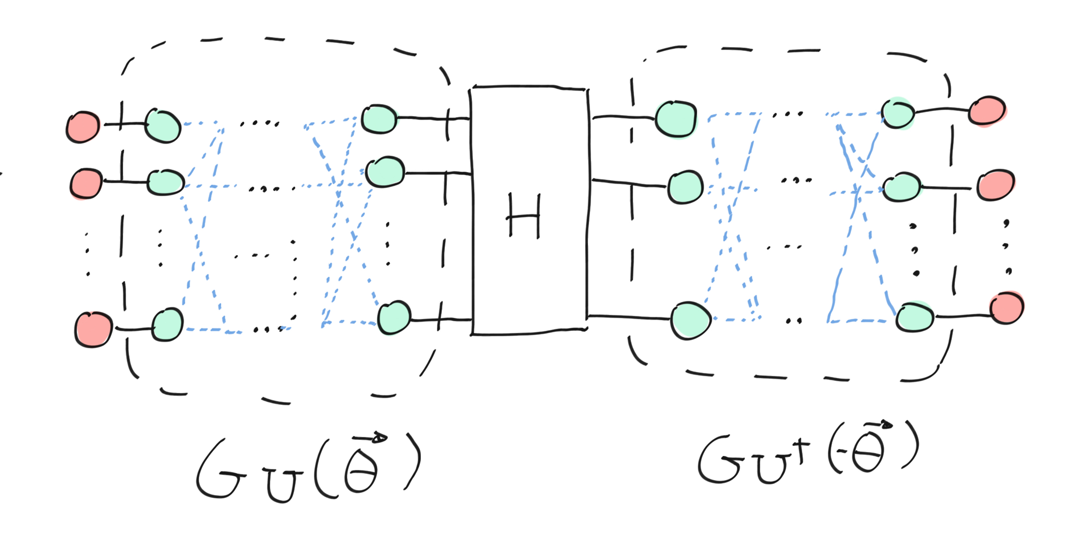
Now we will investigate the partial derivative of the diagram representing the expectation value. The theorem is the following:
Theorem 2: The derivative of the expectation value of a Hamiltonian given a parameterized as a ZX-diagram.
Let’s prove theorem 2, and first we consider a partial derivative on the spider with respect to \(\theta_j\). The spider necessarily appears on both sides, but they have phases of opposite signs and inverse inputs/outputs. By simply writing their definitions and expanding the formula, we obtain:
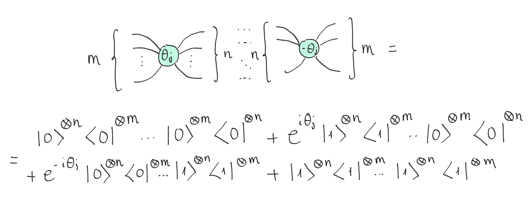
Two Z-spiders depending on the \(j\)-th angle.
Now we have a simple formula where we can easily take the derivative:
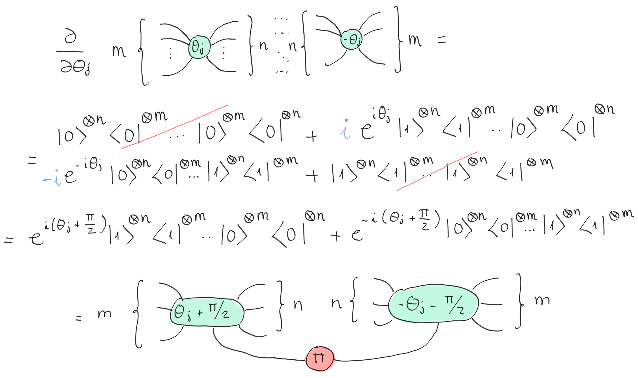
The derivative of two spiders depending on the \(j\)-th angle.
The theorem 2 is proved — we just expressed the partial derivative as a ZX-diagram!
Parameter-shift rule as a ZX-diagram
This theorem can be used to prove the parameter-shift rule. Let’s consider the following ansatz that we transform to its graph-like diagram.
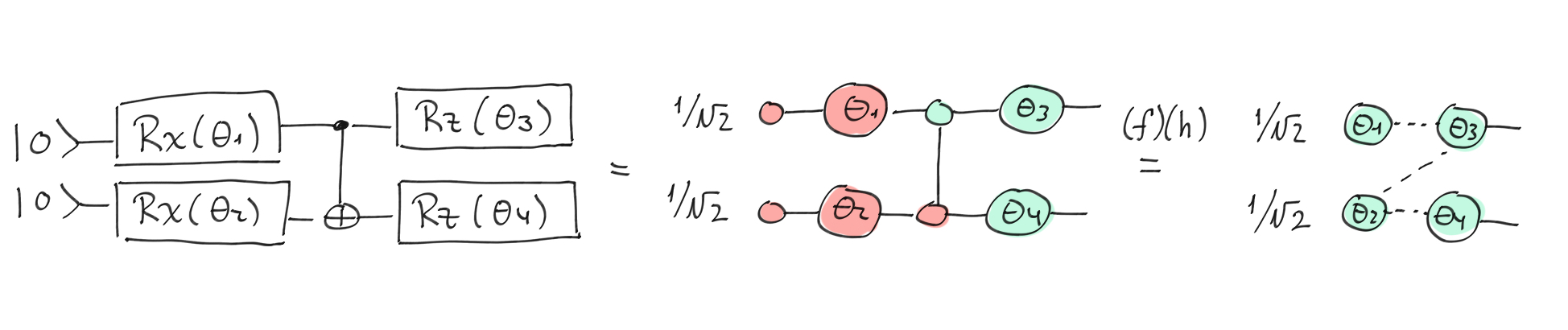
The circuit (on the left) is translated to a ZX-diagram.
The whole circuit is translated to a graph-like ZX-diagram.
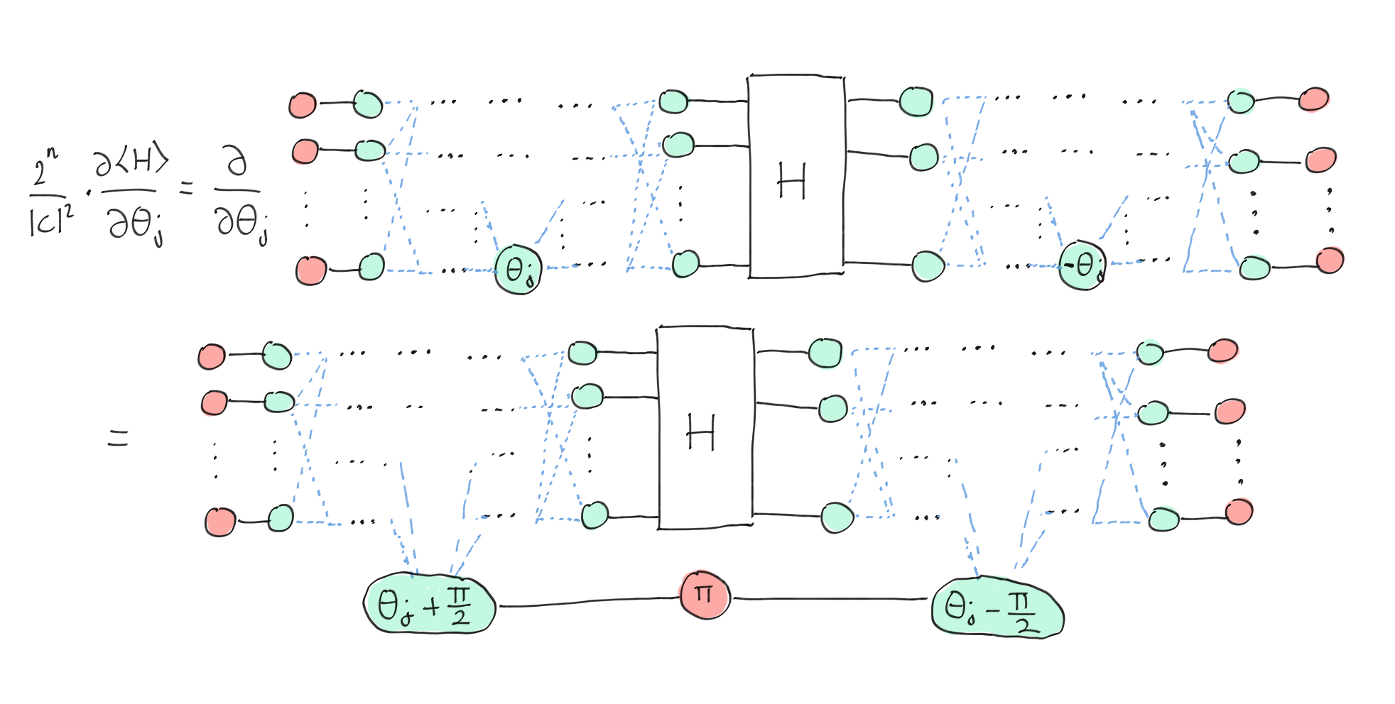
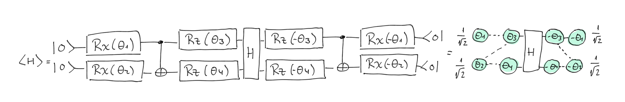
We then apply the previous theorem to get the partial derivative relative to \(\theta_1\).
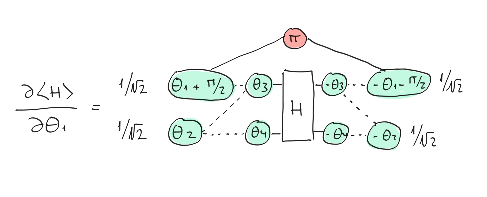
The derivative is applied on the ZX-diagram
The second step is to take the X-spider with phase \(\pi\) and explicitly write the formula \(|+\rangle\langle +| - |-\rangle \langle -|\). We can then separate the diagram into two parts by recalling the definition of the \(|+\rangle\) (phaseless Z-spider) and \(|- \rangle\) (\(2\pi\) Z-spider) states and using the fusion rule for the Z-spider. We obtain the parameter-shift rule!
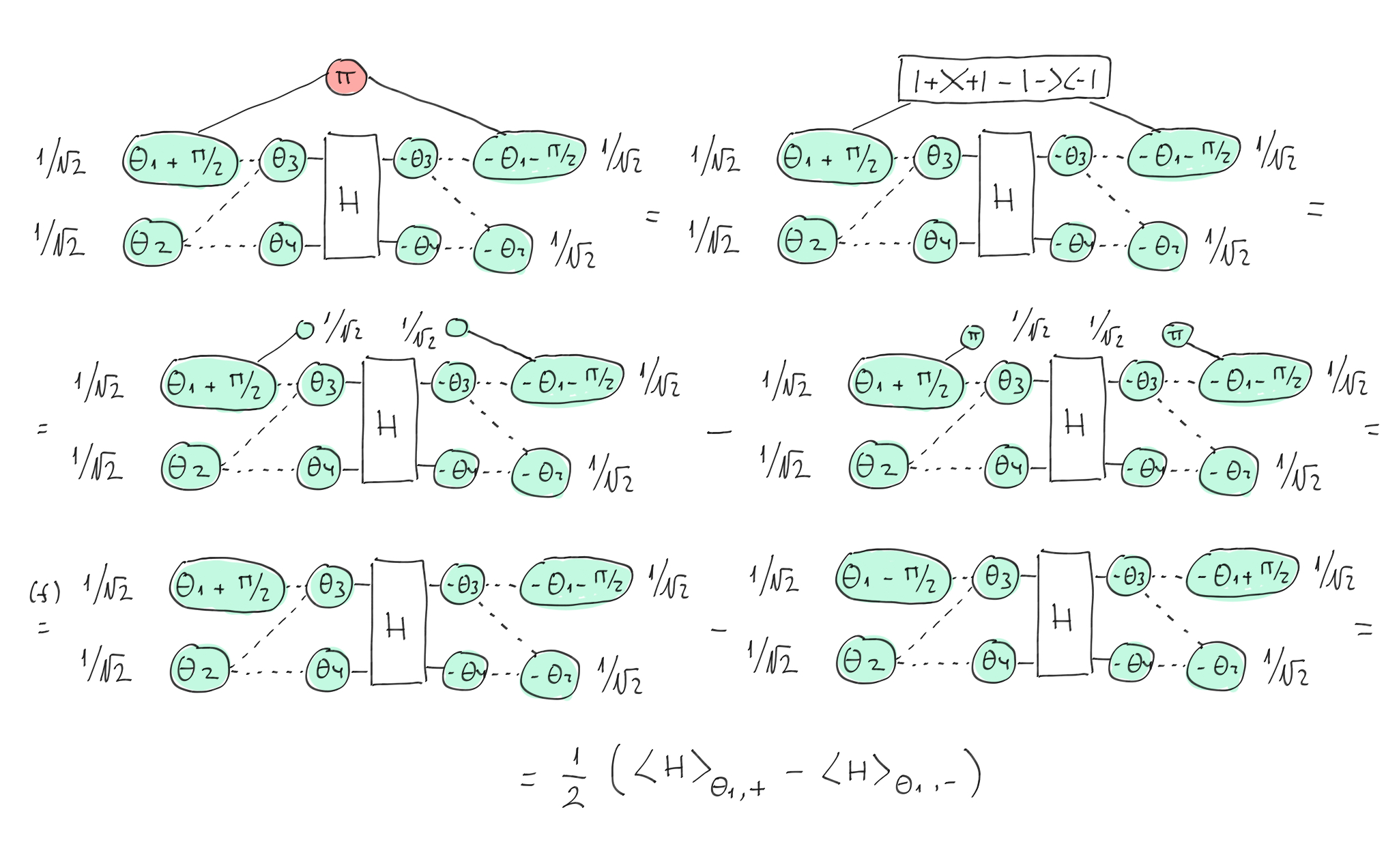
By using theorem 2, we can add an X-spider and shift the phases in the Z-spiders. Then, by explicitly decomposing the spider with the \(|+\rangle\) and \(|-\rangle\) states, we prove the parameter-shift rule!
You can find more information about the differentiation and integration of ZX-diagrams with QML applications in the following paper 6.
ZX-diagrams with PennyLane
Now that we have introduced the formalism of the ZX-calculus, let’s dive into some code and show what you can do with
PennyLane! PennyLane v0.28 added ZX-calculus functionality to the fold. You can use the
to_zx() transform decorator to get a ZX-diagram from a PennyLane
QNode, while from_zx() transforms a ZX-diagram into a PennyLane
tape. We are using the PyZX library 2 under the hood to represent the ZX diagram. Once your circuit is a PyZX
graph, you can draw it, apply some optimization, extract the underlying circuit, and go back to PennyLane.
Let’s start with a very simple circuit consisting of three gates and show that you can represent the
QNode as a PyZX diagram:
import matplotlib.pyplot as plt

import pennylane as qml
import pyzx

dev = qml.device("default.qubit", wires=2)


@qml.transforms.to_zx
@qml.qnode(device=dev)
def circuit():
    qml.PauliX(wires=0),
    qml.PauliY(wires=1),
    qml.CNOT(wires=[0, 1]),
    return qml.expval(qml.PauliZ(wires=0))


g = circuit()
Now that you have a ZX-diagram as a PyZx object, you can use all the tools from the PyZX library to transform the graph. You can simplify the circuit, draw it, and get a new understanding of your quantum computation.
For example, you can use the matplotlib drawer to get a visualization of the diagram. The drawer returns a
matplotlib figure, and therefore you can save it locally with savefig function, or simply show it locally.
fig = pyzx.draw_matplotlib(g)

# The following lines are added because the figure is automatically closed by PyZX.
manager = plt.figure().canvas.manager
manager.canvas.figure = fig
fig.set_canvas(manager.canvas)

plt.show()
You can also take a ZX-diagram in PyZX, convert it into a PennyLane tape and use it in your
QNode. Invoking the PyZX circuit generator:
import random

random.seed(42)
random_circuit = pyzx.generate.CNOT_HAD_PHASE_circuit(qubits=3, depth=10)
print(random_circuit.stats())

graph = random_circuit.to_graph()

tape = qml.transforms.from_zx(graph)
print(tape.operations)
Out:
Circuit  on 3 qubits with 10 gates.
        4 is the T-count
        6 Cliffords among which
        5 2-qubit gates (5 CNOT, 0 other) and
        1 Hadamard gates.
[T(wires=[0]), T(wires=[0]), CNOT(wires=[2, 0]), T(wires=[2]), CNOT(wires=[1, 0]), CNOT(wires=[0, 2]), T(wires=[2]), Hadamard(wires=[0]), CNOT(wires=[2, 1]), CNOT(wires=[2, 1])]
We get a tape corresponding to the randomly generated circuit that we can use in any QNode. This
functionality will be very useful for our next topic: circuit optimization.
Diagram optimization and circuit extraction
The ZX-calculus is more general and more flexible than the usual circuit representation. We can therefore represent circuits with ZX-diagrams and apply rewriting rules to simplify them — like we did for teleportation. But, not every ZX-diagram has a corresponding circuit. To get back to circuits, a method for circuit extraction is needed. For a rigorous introduction to this active and promising field of application, see 7. The basic idea is captured below:
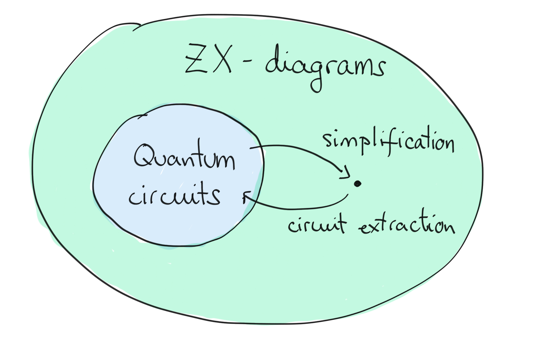
To simplify ZX-diagrams, not only can we use the rewriting rules defined previously, but we can also use graph-theoretic transformations called local complementation and pivoting. These are special transformations that can only be applied to “graph-like” ZX-diagrams. As defined in 7, a ZX-diagram is graph-like if
All spiders are Z-spiders.
Z-spiders are only connected via Hadamard edges.
There are no parallel Hadamard edges or self-loops.
Every input or output is connected to a Z-spider and every Z-spider is connected to at most one input or output.
A ZX-diagram is called a graph state if it is graph-like: every spider is connected to an output and there are no phaseless spiders. Furthermore, it was proved that every ZX-diagram is equal to a graph-like ZX-diagram. Thus, after conversion into graph-like form, we can use graph-theoretic tools on all ZX-diagrams.
The basic idea is to use the graph-theoretic transformations to get rid of as many interior spiders as possible. Interior spiders are the one without inputs or outputs connected to them. We introduce some names for the spiders depending on their phases:
A Pauli spider has a phase that is a multiple of \(\pi\).
A Clifford spider has a phase that is a multiple of \(\frac{\pi}{2}\).
A proper Clifford spider is a Clifford spider with a phase which is an odd multiple of \(\frac{\pi}{2}\).
Theorem 5.4 in 7 provides an algorithm which takes a graph-like diagram and performs the following:
Remove all interior proper Clifford spiders,
Remove adjacent pairs of interior Pauli spiders,
Remove interior Pauli spiders adjacent to a boundary spider.
This procedure is implemented in PyZX as the full_reduce() function. The complexity of the procedure is
\(\mathcal{O}(n^3)\), where \(n\) is the number of spiders. Let’s create an example with the circuit
mod_5_4. The circuit
\(63\) gates: \(28\) T. gates, \(28\) CNOT, \(6\)
Hadamard and \(1\) PauliX.
dev = qml.device("default.qubit", wires=5)


@qml.transforms.to_zx
@qml.qnode(device=dev)
def mod_5_4():
    qml.PauliX(wires=4),
    qml.Hadamard(wires=4),
    qml.CNOT(wires=[3, 4]),
    qml.adjoint(qml.T(wires=[4])),
    qml.CNOT(wires=[0, 4]),
    qml.T(wires=[4]),
    qml.CNOT(wires=[3, 4]),
    qml.adjoint(qml.T(wires=[4])),
    qml.CNOT(wires=[0, 4]),
    qml.T(wires=[3]),
    qml.T(wires=[4]),
    qml.CNOT(wires=[0, 3]),
    qml.T(wires=[0]),
    qml.adjoint(qml.T(wires=[3]))
    qml.CNOT(wires=[0, 3]),
    qml.CNOT(wires=[3, 4]),
    qml.adjoint(qml.T(wires=[4])),
    qml.CNOT(wires=[2, 4]),
    qml.T(wires=[4]),
    qml.CNOT(wires=[3, 4]),
    qml.adjoint(qml.T(wires=[4])),
    qml.CNOT(wires=[2, 4]),
    qml.T(wires=[3]),
    qml.T(wires=[4]),
    qml.CNOT(wires=[2, 3]),
    qml.T(wires=[2]),
    qml.adjoint(qml.T(wires=[3]))
    qml.CNOT(wires=[2, 3]),
    qml.Hadamard(wires=[4]),
    qml.CNOT(wires=[3, 4]),
    qml.Hadamard(wires=4),
    qml.CNOT(wires=[2, 4]),
    qml.adjoint(qml.T(wires=[4])),
    qml.CNOT(wires=[1, 4]),
    qml.T(wires=[4]),
    qml.CNOT(wires=[2, 4]),
    qml.adjoint(qml.T(wires=[4])),
    qml.CNOT(wires=[1, 4]),
    qml.T(wires=[4]),
    qml.T(wires=[2]),
    qml.CNOT(wires=[1, 2]),
    qml.T(wires=[1]),
    qml.adjoint(qml.T(wires=[2]))
    qml.CNOT(wires=[1, 2]),
    qml.Hadamard(wires=[4]),
    qml.CNOT(wires=[2, 4]),
    qml.Hadamard(wires=4),
    qml.CNOT(wires=[1, 4]),
    qml.adjoint(qml.T(wires=[4])),
    qml.CNOT(wires=[0, 4]),
    qml.T(wires=[4]),
    qml.CNOT(wires=[1, 4]),
    qml.adjoint(qml.T(wires=[4])),
    qml.CNOT(wires=[0, 4]),
    qml.T(wires=[4]),
    qml.T(wires=[1]),
    qml.CNOT(wires=[0, 1]),
    qml.T(wires=[0]),
    qml.adjoint(qml.T(wires=[1])),
    qml.CNOT(wires=[0, 1]),
    qml.Hadamard(wires=[4]),
    qml.CNOT(wires=[1, 4]),
    qml.CNOT(wires=[0, 4]),
    return qml.expval(qml.PauliZ(wires=0))


g = mod_5_4()
pyzx.simplify.full_reduce(g)

fig = pyzx.draw_matplotlib(g)

# The following lines are added because the figure is automatically closed by PyZX.
manager = plt.figure().canvas.manager
manager.canvas.figure = fig
fig.set_canvas(manager.canvas)

plt.show()
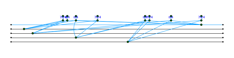
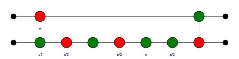
We see that after applying the procedure, we end up with only 16 interior Z-spiders and 5 boundary spiders. We also see that all non-Clifford phases appear on the interior spiders. The simplification procedure was successful, but we have a graph-like ZX-diagram with no quantum circuit equivalent. We need to extract a circuit!
The extraction of circuits is a highly non-trivial task and can be a #P-hard problem as shown in this paper 9 by de Beaudrap et al . There are two different algorithms introduced in the same paper. First, for Clifford circuits, the procedure will erase all interior spiders, and the diagram is left in a graph-state from which a Clifford circuit can be extracted using a total of eight layers with only one layer of CNOTs.
For non-Clifford circuits, the problem is more complex because we are left with non-Clifford interior spiders. From
the diagram produced by the simplification procedure, the extraction progresses through the diagram from
right-to-left, consuming gates on the left and adding gates on the right. It produces better results than other
cut-and-resynthesize techniques. The extraction procedure is implemented in PyZX as the function
pyzx.circuit.extract_circuit. We can apply this procedure to the example mod_5_4 above:
circuit_extracted = pyzx.extract_circuit(g.copy())
print(circuit_extracted.stats())
Out:
Circuit  on 5 qubits with 56 gates.
        8 is the T-count
        48 Cliffords among which
        22 2-qubit gates (0 CNOT, 22 other) and
        26 Hadamard gates.
Example: T-count optimization
A concrete application of these ZX optimization techniques is the reduction of the expensive non-Clifford T-count of a quantum circuit. Indeed, T-count optimization is an area where the ZX-calculus has shown very good results 8 .
Let’s start by using with the mod_5_4 circuit introduced above. We applied the to_zx()
decorator in order to transform our circuit to a ZX graph. You can get this PyZX graph by calling the
QNode:
g = mod_5_4()
t_count = pyzx.tcount(g)
print("T count before optimization:", t_count)
Out:
T count before optimization: 28
PyZX gives multiple options for optimizing ZX graphs: full_reduce() and teleport_reduce()
to name a couple. The full_reduce() applies all optimization passes, but the final result may not be
circuit-like. Converting back to a quantum circuit from a fully reduced graph might be difficult or impossible.
Therefore, we instead recommend using teleport_reduce(), as it preserves the diagram structure.
Because of this, the circuit does not need to be extracted and can be directly sent back to PennyLane. Let’s see
how it works:
g = pyzx.simplify.teleport_reduce(g.copy())
opt_t_count = pyzx.tcount(g)
print("T count after optimization:", opt_t_count)
Out:
T count after optimization: 8
The from_zx() transform converts the optimized circuit back into PennyLane format,
and which is made possible because we used pyzx.teleport_reduce and do not need to extract
the circuit.
qscript_opt = qml.transforms.from_zx(g)

wires = qml.wires.Wires([4, 3, 0, 2, 1])
wires_map = dict(zip(qscript_opt.wires, wires))
qscript_opt_reorder = qml.map_wires(input=qscript_opt, wire_map=wires_map)


@qml.qnode(device=dev)
def mod_5_4():
    for o in qscript_opt_reorder:
        qml.apply(o)
    return qml.expval(qml.PauliZ(wires=0))


specs = qml.specs(mod_5_4)()

print("Number of quantum gates:", specs["num_operations"])
print("Circuit gates:", specs["gate_types"])
Out:
Number of quantum gates: 53
Circuit gates: defaultdict(<class 'int'>, {'PauliX': 1, 'Hadamard': 6, 'CNOT': 28, 'T': 4, 'S': 6, 'Adjoint(T)': 4, 'Adjoint(S)': 4})
We have reduced the T-count! Taking a full census, the circuit contains \(53\) gates: \(8\)
T gates, \(28\) CNOT, \(6\) Hadamard,
\(1\) PauliX and \(10\) S. We successfully reduced the T-count by
20 and have 10 additional S gates. The number of CNOT gates remained the
same.
Conclusion
Now that you have read this tutorial, you should be able to use the ZX-calculus to solve your quantum problems. You can describe quantum circuits with the ZX-spiders and the H-box and create ZXH-diagrams. Furthermore, you can use the simplifying rules to get another view of the underlying structure of your circuit. We have proved its utility for optimizing quantum circuits and shown that the ZX-calculus is more than promising for quantum machine learning. It was not covered in this introduction, but the ZX-calculus can also be used for quantum-error correction — it’s no wonder why some quantum physicists call ZX-calculus the “Swiss army knife” of quantum computing tools!
Acknowledgement
The author would also like to acknowledge the helpful inputs of Richard East, David Wakeham and Isaac De Vlugt. The author is also thankful for the beautiful drawings by Guillermo Alonso and for the great thumbnail and teleportation gif by Tarik El-Khateeb.
References
- 1(1,2)
Bob Coecke and Ross Duncan. “Interacting Quantum Observables: Categorical Algebra and Diagrammatics.” ArXiv.
- 2(1,2)
John van de Wetering. “PyZX.” PyZX GitHub.
- 3(1,2,3)
Richard D. P. East, John van de Wetering, Nicholas Chancellor and Adolfo G. Grushin. “AKLT-states as ZX-diagrams: diagrammatic reasoning for quantum states.” ArXiv.
- 4(1,2,3,4,5,6,7)
John van de Wetering. “ZX-calculus for the working quantum computer scientist.” ArXiv.
- 5(1,2)
Chen Zhao and Xiao-Shan Gao. “Analyzing the barren plateau phenomenon in training quantum neural networks with the ZX-calculus” Quantum Journal.
- 6
Quanlong Wang, Richie Yeung, and Mark Koch. “Differentiating and Integrating ZX Diagrams with Applications to Quantum Machine Learning” Quantum Journal.
- 7(1,2,3,4)
Ross Duncan, Aleks Kissinger, Simon Perdrix, and John van de Wetering. “Graph-theoretic Simplification of Quantum Circuits with the ZX-calculus.” Quantum Journal.
- 8
Aleks Kissinger and John van de Wetering. “Reducing T-count with the ZX-calculus.” ArXiv.
- 9
Niel de Beaudrap, Aleks Kissinger and John van de Wetering. “Circuit Extraction for ZX-diagrams can be #P-hard.” ArXiv.