Estimating observables with classical shadows in the Pauli basis

Author: Korbinian Kottmann — Posted: 07 October 2022. Last updated: 11 October 2022.

We briefly introduce the classical shadow formalism in the Pauli basis and showcase PennyLane’s new implementation of it. Classical shadows are sometimes believed to provide advantages in quantum resources to simultaneously estimate multiple observables. We demystify this misconception and perform fair comparisons between classical shadow measurements and simultaneously measuring qubit-wise-commuting observable groups.

Classical shadow theory

A classical shadow is a classical description of a quantum state that is capable of reproducing expectation values of local Pauli observables, see 1. We briefly go through their theory here, and note the two additional demos in Classical shadows and Machine learning for quantum many-body problems.

We are here focussing on the case where measurements are performed in the Pauli basis. The idea of classical shadows is to measure each qubit in a random Pauli basis. While doing so, one keeps track of the performed measurement (its recipes) in form of integers [0, 1, 2] corresponding to the measurement bases [X, Y, Z], respectively. At the same time, the measurement outcome (its bits) are recorded, where [0, 1] corresponds to the eigenvalues [1, -1], respectively.

We record \(T\) of such measurements, and for the \(t\)-th measurement, we can reconstruct the local_snapshot for \(n\) qubits via

\[\rho^{(t)} = \bigotimes_{i=1}^{n} 3 U^\dagger_i |b^{(t)}_i \rangle \langle b^{(t)}_i | U_i - \mathbb{I},\]

where \(U_i\) is the diagonalizing rotation for the respective Pauli basis (e.g. \(U_i=H\) for measurement in \(X\)) for qubit i. \(|b^{(t)}_i\rangle = (1 - b^{(t)}_i, b^{(t)}_i)\) is the corresponding computational basis state given by the output bit \(b^{(t)}_i \in \{0, 1\}\).

From these local snapshots, one can compute expectation values of q-local Pauli strings, where locality refers to the number of non-Identity operators. The expectation value of any Pauli string \(\bigotimes_iO_i\) with \(O_i \in \{X, Y, Z, \mathbb{I}\}\) can be estimated by computing

\[\Big\langle \bigotimes_iO_i \Big\rangle = \frac{1}{T} \sum_{t=1}^T \text{tr}\left[ \rho^{(t)} \left(\bigotimes_i O_i\right) \right].\]

Error bounds given by the number of measurements \(T = \mathcal{O}\left( \log(M) 4^q/\varepsilon^2 \right)\) guarantee that sufficiently many correct measurements were performed to estimate \(M\) different observables up to additive error \(\varepsilon\). This \(\log(M)\) factor may lead one to think that with classical shadows one can magically estimate multiple observables at a lower cost than with direct measurement. We resolve this misconception in the following section.

Unraveling the mystery

Using algebraic properties of Pauli operators, we show how to exactly compute the above expression from just the bits and recipes without explicitly reconstructing any snapshots. This gives us insights to what is happening under the hood and how the T measuerements are used to estimate the observable.

Let us start by looking at individual snapshot expectation values \(\langle \bigotimes_iO_i \rangle ^{(t)} = \text{tr}\left[\rho^{(t)} \left(\bigotimes_iO_i \right)\right]\). First, we convince ourselves of the identity

\[U_i^\dagger |b^{(t)}_i\rangle \langle b^{(t)}_i| U_i = \frac{1}{2}\left((1-2b^{(t)}_i) P_i + \mathbb{I}\right),\]

where \(P_i \in \{X, Y, Z\}\) is the Pauli operator corresponding to \(U_i\) (note that in this case \(P_i\) is never the identity). The snapshot expectation value then reduces to

\[\Big\langle\bigotimes_iO_i\Big\rangle^{(t)} = \prod_{i=1}^n \text{tr}\left[\frac{3}{2}(1-2b^{(t)}_i)P_i O_i + \frac{1}{2}O_i\right].\]

For that trace we find three different cases. The cases where \(O_i=\mathbb{I}\) yield a trivial factor \(1\) to the product. The full product is always zero if any of the non-trivial \(O_i\) do not match \(P_i\). So in total, only in the case that all \(q\) Pauli operators match, we find

\[\Big\langle\bigotimes_iO_i\Big\rangle^{(t)} = 3^q \prod_{\text{i non-trivial}}(1-2b^{(t)}_i).\]

This implies that in order to compute the expectation value of a Pauli string

\[\Big\langle\bigotimes_iO_i\Big\rangle = \frac{1}{\tilde{T}} \sum_{\tilde{t}} \prod_{\text{i non-trivial}}(1-2b^{(t)}_i)\]

we simply need average over the product of \(1 - 2b^{(t)}_i = \pm 1\) for those \(\tilde{T}\) snapshots where the measurement recipe matches the observable, indicated by the special index \(\tilde{t}\) for the matching measurements. Note that the probability of a match is \(1/3^q\) such that we have \(\tilde{T} \approx T / 3^q\) on average.

This implies that computing expectation values with classical shadows comes down to picking the specific subset of snapshots where those specific observables were already measured and discarding the remaining. If the desired observables are known prior to the measurement, one is thus advised to directly perform those measurements. This was referred to as derandomization by the authors in a follow-up paper 2.

We will later compare the naive classical shadow approach to directly measuring the desired observables and make use of simultaneously measuring qubit-wise-commuting observables. Before that, let us demonstrate how to perform classical shadow measurements in a differentiable manner in PennyLane.

PennyLane implementation

There are two ways of computing expectation values with classical shadows in PennyLane. The first is to return qml.shadow_expval directly from the qnode. This has the advantage that it preserves the typical PennyLane syntax and is differentiable.

import pennylane as qml
import pennylane.numpy as np
from matplotlib import pyplot as plt
from pennylane import classical_shadow, shadow_expval, ClassicalShadow

np.random.seed(666)

H = qml.Hamiltonian([1., 1.], [qml.PauliZ(0) @ qml.PauliZ(1), qml.PauliX(0) @ qml.PauliX(1)])

dev = qml.device("default.qubit", wires=range(2), shots=10000)
@qml.qnode(dev, interface="autograd")
def qnode(x, H):
    qml.Hadamard(0)
    qml.CNOT((0,1))
    qml.RX(x, wires=0)
    return shadow_expval(H)

x = np.array(0.5, requires_grad=True)

Compute expectation values and derivatives thereof in the common way in PennyLane.

print(qnode(x, H), qml.grad(qnode)(x, H))

Out:

1.881 -0.4454999999999999

Each call of qml.shadow_expval performs the number of shots dictated by the device. So to avoid unnecessary device executions you can provide a list of observables to qml.shadow_expval.

Hs = [H, qml.PauliX(0), qml.PauliY(0), qml.PauliZ(0)]
print(qnode(x, Hs))
print(qml.jacobian(qnode)(x, Hs))

Out:

[ 1.863  -0.0114 -0.0096 -0.0072]
[-0.4905 -0.0075  0.0093  0.0009]

Alternatively, you can compute expectation values by first performing the shadow measurement and then perform classical post-processing using the ClassicalShadow class methods.

dev = qml.device("default.qubit", wires=range(2), shots=1000)
@qml.qnode(dev, interface="autograd")
def qnode(x):
    qml.Hadamard(0)
    qml.CNOT((0,1))
    qml.RX(x, wires=0)
    return classical_shadow(wires=range(2))

bits, recipes = qnode(0.5)
shadow = ClassicalShadow(bits, recipes)
print(bits.shape, recipes.shape)

Out:

(1000, 2) (1000, 2)

After recording these T=1000 quantum measurements, we can post-process the results to arbitrary local expectation values of Pauli strings. For example, we can compute the expectation value of a Pauli string

print(shadow.expval(qml.PauliX(0) @ qml.PauliX(1)))

Out:

0.927

or of a Hamiltonian:

H = qml.Hamiltonian([1., 1.], [qml.PauliZ(0) @ qml.PauliZ(1), qml.PauliX(0) @ qml.PauliX(1)])
print(shadow.expval(H))

Out:

1.764

This way of computing expectation values is not automatically differentiable in PennyLane though.

Comparing quantum resources with conventional measurement methods

The goal of the following section is to compare estimation accuracy for a given number of quantum executions with more conventional methods like simultaneously measuring qubit-wise-commuting (qwc) groups, see Measurement optimization. We are going to look at three different cases: The two extreme scenarios of measuring one single and all q-local Pauli strings, as well as the more realistic scenario of measuring a molecular Hamiltonian. We find that for a fix budget of measurements, one is almost never advised to use classical shadows for estimating expectation values.

Measuring one single observable

We start with the case of one single measurement. From the analysis above it should be quite clear that in the case of random Pauli measurement in the classical shadows formalism, a lot of quantum resources are wasted as all the measurements that do not match the observable are discarded. This is certainly not what classical shadows were intended for in the first place, but it helps to stress the point of wasted measurements.

We start by fixing a circuit and an observable, for which we compute the exact result for infinite shots.

def rmsd(x, y):
    """root mean square difference"""
    return np.sqrt(np.mean((x - y)**2))

n_wires = 10

x = np.arange(2*n_wires, dtype="float64")
def circuit():
    for i in range(n_wires):
        qml.RY(x[i], i)
    for i in range(n_wires-1):
        qml.CNOT((i, i+1))
    for i in range(n_wires):
        qml.RY(x[i+n_wires], i)

obs = qml.PauliX(0) @ qml.PauliZ(3) @ qml.PauliX(6) @ qml.PauliZ(7)

dev_ideal = qml.device("default.qubit", wires=range(n_wires), shots=None)
@qml.qnode(dev_ideal, interface="autograd")
def qnode_ideal():
    circuit()
    return qml.expval(obs)

exact = qnode_ideal()

We now compare estimating the observable with classical shadows vs the canonical estimation.

finite = []
shadow = []
shotss = range(100, 1000, 100)
for shots in shotss:
    for _ in range(10):
        # repeating experiment 10 times to obtain averages and standard deviations
        dev = qml.device("default.qubit", wires=range(10), shots=shots)

        @qml.qnode(dev, interface="autograd")
        def qnode_finite():
            circuit()
            return qml.expval(obs)

        @qml.qnode(dev, interface="autograd")
        def qnode_shadow():
            circuit()
            return qml.shadow_expval(obs)

        finite.append(rmsd(qnode_finite(), exact))
        shadow.append(rmsd(qnode_shadow(), exact))


dq = np.array(finite).reshape(len(shotss), 10)
dq, ddq = np.mean(dq, axis=1), np.var(dq, axis=1)
ds = np.array(shadow).reshape(len(shotss), 10)
ds, dds = np.mean(ds, axis=1), np.var(ds, axis=1)

plt.errorbar(shotss, ds, yerr=dds, fmt="x-", label="shadow")
plt.errorbar(shotss, dq, yerr=ddq, fmt="x-", label="direct")
plt.xlabel("total number of shots T", fontsize=20)
plt.ylabel("Error (RMSD)", fontsize=20)
plt.legend()
plt.tight_layout()
plt.show()

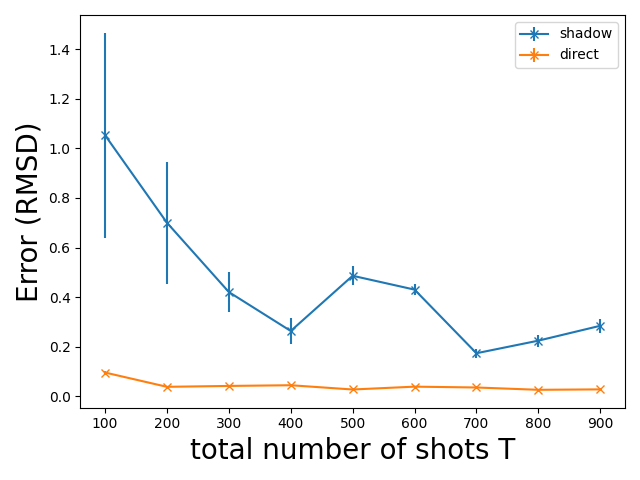
Unsurprisingly, the deviation is consistently smaller by directly measuring the observable since we are not discarding any measurement results.

All q-local observables

For the case of measuring all q-local Pauli strings we expect both strategies to yield more or less the same results. In this extreme case, no measurements are discarded in the classical shadow protocol. Let us put that to test. First, we generate a list of all q-local observables for n qubits.

from itertools import product, combinations
from functools import reduce

all_observables = []
n = 5
q = 2
# create all combination of q entries of range(n)
for w in combinations(range(n), q):
    # w = [0, 1], [0, 2], .., [1, 2], [1, 3], .., [n-1, n]
    observables = []

    # Create all combinations of possible Pauli products P_i P_j P_k.... for wires w
    for obs in product(
        *[[qml.PauliX, qml.PauliY, qml.PauliZ] for _ in range(len(w))]
        ):
        # Perform tensor product (((P_i @ P_j) @ P_k ) @ ....)
        observables.append(reduce(lambda a, b: a @ b, [ob(wire) for ob, wire in zip(obs, w)]))
    all_observables.extend(observables)

for observable in all_observables[:10]:
    print(observable)

Out:

PauliX(wires=[0]) @ PauliX(wires=[1])
PauliX(wires=[0]) @ PauliY(wires=[1])
PauliX(wires=[0]) @ PauliZ(wires=[1])
PauliY(wires=[0]) @ PauliX(wires=[1])
PauliY(wires=[0]) @ PauliY(wires=[1])
PauliY(wires=[0]) @ PauliZ(wires=[1])
PauliZ(wires=[0]) @ PauliX(wires=[1])
PauliZ(wires=[0]) @ PauliY(wires=[1])
PauliZ(wires=[0]) @ PauliZ(wires=[1])
PauliX(wires=[0]) @ PauliX(wires=[2])

We now group these into qubit-wise-commuting (qwc) groups using group_observables() to learn the number of groups. We need this number to make a fair comparison with classical shadows as we allow for only T/n_groups shots per group, such that the total number of shots is the same as for the classical shadow execution. We again compare both approaches.

n_groups = len(qml.pauli.group_observables(all_observables))

dev_ideal = qml.device("default.qubit", wires=range(n), shots=None)

x = np.random.rand(n*2)
def circuit():
    for i in range(n):
        qml.RX(x[i], i)

    for i in range(n):
        qml.CNOT((i, (i+1)%n))

    for i in range(n):
        qml.RY(x[i+n], i)

    for i in range(n):
        qml.CNOT((i, (i+1)%n))

@qml.qnode(dev_ideal, interface="autograd")
def qnode_ideal():
    circuit()
    return qml.expval(H)

exact = qnode_ideal()
finite = []
shadow = []
shotss = range(100, 10000, 2000)
for shots in shotss:
    # random Hamiltonian with all q-local observables
    coeffs = np.random.rand(len(all_observables))
    H = qml.Hamiltonian(coeffs, all_observables, grouping_type="qwc")

    @qml.qnode(dev_ideal, interface="autograd")
    def qnode_ideal():
        circuit()
        return qml.expval(H)

    exact = qnode_ideal()

    for _ in range(10):
        dev = qml.device("default.qubit", wires=range(5), shots=shots)

        @qml.qnode(dev, interface="autograd")
        def qnode_finite():
            circuit()
            return qml.expval(H)

        dev = qml.device("default.qubit", wires=range(5), shots=shots*n_groups)
        @qml.qnode(dev, interface="autograd")
        def qnode_shadow():
            circuit()
            return qml.shadow_expval(H)

        finite.append(rmsd(qnode_finite(), exact))
        shadow.append(rmsd(qnode_shadow(), exact))


dq = np.array(finite).reshape(len(shotss), 10)
dq, ddq = np.mean(dq, axis=1), np.var(dq, axis=1)
ds = np.array(shadow).reshape(len(shotss), 10)
ds, dds = np.mean(ds, axis=1), np.var(ds, axis=1)
plt.errorbar(shotss, ds, yerr=dds, fmt="x-", label="shadow")
plt.errorbar(shotss, dq, yerr=ddq, fmt="x-", label="qwc")
plt.xlabel("total number of shots T", fontsize=20)
plt.ylabel("Error (RMSD)", fontsize=20)
plt.legend()
plt.tight_layout()
plt.show()

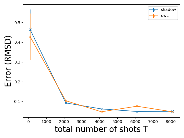
We see that as expected the performance is more or less the same since no quantum measurements are discarded for the shadows in this case. Depending on the chosen random seed there are quantitative variations to this image, but the overall qualitative result remains the same.

Molecular Hamiltonians

We now look at the more realistic case of measuring a molecular Hamiltonian. We tak \(\text{H}_2\text{O}\) as an example. You can find more details on this Hamiltonian in Building molecular Hamiltonians. We start by building the Hamiltonian and enforcing qwc groups by setting grouping_type='qwc'.

symbols = ["H", "O", "H"]
coordinates = np.array([-0.0399, -0.0038, 0.0, 1.5780, 0.8540, 0.0, 2.7909, -0.5159, 0.0])

basis_set = "sto-3g"
H, n_wires = qml.qchem.molecular_hamiltonian(
    symbols,
    coordinates,
    charge=0,
    mult=1,
    basis=basis_set,
    active_electrons=4,
    active_orbitals=4,
    mapping="bravyi_kitaev",
    method="pyscf",
)

coeffs, obs = H.coeffs, H.ops
H_qwc = qml.Hamiltonian(coeffs, obs, grouping_type="qwc")

groups = qml.pauli.group_observables(obs)
n_groups = len(groups)
print(f"number of ops in H: {len(obs)}, number of qwc groups: {n_groups}")
print(f"Each group has sizes {[len(_) for _ in groups]}")

Out:

number of ops in H: 193, number of qwc groups: 50
Each group has sizes [5, 2, 4, 1, 3, 2, 2, 5, 2, 5, 4, 5, 4, 3, 5, 5, 3, 3, 6, 3, 2, 2, 2, 2, 2, 4, 2, 3, 4, 1, 2, 4, 4, 3, 6, 4, 4, 4, 6, 2, 4, 2, 7, 2, 8, 4, 7, 3, 13, 8]

We use a pre-prepared Ansatz that approximates the \(\text{H}_2\text{O}\) ground state for the given geometry. You can construct this Ansatz by running VQE, see A brief overview of VQE. We ran this once on an ideal simulator to get the exact result of the energy for the given Ansatz.

singles, doubles = qml.qchem.excitations(electrons=4, orbitals=n_wires)
hf = qml.qchem.hf_state(4, n_wires)
theta = np.array([ 2.20700008e-02,  8.29716448e-02,  2.19227085e+00,
    3.19128513e+00, -1.35370403e+00,  6.61615333e-03,
    7.40317830e-01, -3.73367029e-01,  4.35206518e-02,
    -1.83668679e-03, -4.59312535e-03, -1.91103984e-02,
    8.21320961e-03, -1.48452294e-02, -1.88176061e-03,
    -1.66141213e-02, -8.94505652e-03,  6.92045656e-01,
    -4.54217610e-04, -8.22532179e-04,  5.27283799e-03,
    6.84640451e-03,  3.02313759e-01, -1.23117023e-03,
    4.42283398e-03,  6.02542038e-03])

res_exact = -74.57076341
def circuit():
    qml.AllSinglesDoubles(weights = theta,
        wires = range(n_wires),
        hf_state = hf,
        singles = singles,
        doubles = doubles)

We again follow the same simple strategy of giving each group the same number of shots T/n_groups for T total shots.

d_qwc = []
d_sha = []

shotss = np.arange(20, 220, 20)

for shots in shotss:
    for _ in range(10):

        # execute qwc measurements
        dev_finite = qml.device("default.qubit", wires=range(n_wires), shots=int(shots))
        @qml.qnode(dev_finite, interface="autograd")
        def qnode_finite(H):
            circuit()
            return qml.expval(H)

        with qml.Tracker(dev_finite) as tracker_finite:
            res_finite = qnode_finite(H_qwc)

        # execute shadows measurements
        dev_shadow = qml.device("default.qubit", wires=range(n_wires), shots=int(shots)*n_groups)
        @qml.qnode(dev_shadow, interface="autograd")
        def qnode():
            circuit()
            return classical_shadow(wires=range(n_wires))

        with qml.Tracker(dev_shadow) as tracker_shadows:
            bits, recipes = qnode()

        shadow = ClassicalShadow(bits, recipes)
        res_shadow = shadow.expval(H, k=1)

        # Guarantuee that we are not cheating and its a fair fight
        assert tracker_finite.totals["shots"] <=  tracker_shadows.totals["shots"]

        d_qwc.append(rmsd(res_finite, res_exact))
        d_sha.append(rmsd(res_shadow, res_exact))


dq = np.array(d_qwc).reshape(len(shotss), 10)
dq, ddq = np.mean(dq, axis=1), np.var(dq, axis=1)
ds = np.array(d_sha).reshape(len(shotss), 10)
ds, dds = np.mean(ds, axis=1), np.var(ds, axis=1)
plt.errorbar(shotss*n_groups, ds, yerr=dds, fmt="x-", label="shadow")
plt.errorbar(shotss*n_groups, dq, yerr=ddq, fmt="x-", label="qwc")
plt.xlabel("total number of shots T", fontsize=20)
plt.ylabel("Error (RMSD)", fontsize=20)
plt.legend()
plt.tight_layout()
plt.show()

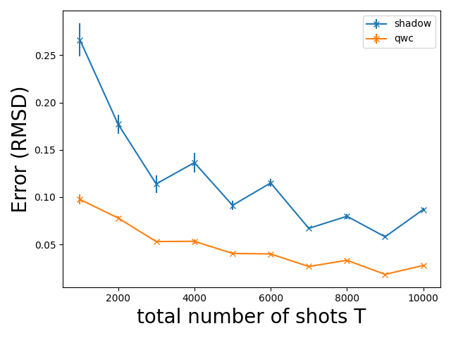
For this realistic example, one is clearly better advised to directly compute the expectation values and not waste precious quantum resources on unused measurements in the classical shadow protocol.

Conclusion

Overall, we saw that classical shadows always waste unused quantum resources for measurements that are not used, except some extreme cases. For the rare case that the observables that are to be determined are not known before the measurement, classical shadows may prove advantageous.

We have been using a relatively simple approach to qwc grouping, as group_observables() is based on the largest first (LF) heuristic (see largest_first()). There has been intensive research in recent years on optimizing qwc measurement schemes. Similarily, it has been realized by the original authors that the randomized shadow protocol can be improved by what they call derandomization 2. Currently, it seems advanced grouping algorithms are still the preferred choice, as is illustrated and discused in 3.

References

1

Hsin-Yuan Huang, Richard Kueng, John Preskill “Predicting Many Properties of a Quantum System from Very Few Measurements.” arXiv:2002.08953, 2020.

2(1,2)

Hsin-Yuan Huang, Richard Kueng, John Preskill “Efficient estimation of Pauli observables by derandomization.” arXiv:2103.07510, 2021.

3

Tzu-Ching Yen, Aadithya Ganeshram, Artur F. Izmaylov “Deterministic improvements of quantum measurements with grouping of compatible operators, non-local transformations, and covariance estimates.” arXiv:2201.01471, 2022.

About the author

Korbinian Kottmann

Korbinian is a Quantum Scientist at Xanadu, interested in quantum simulation and quantum software.

demos/tutorial_diffable_shadows

 

Download Python script

 

Download Notebook

 

View on GitHub