Quantum natural SPSA optimizer

Author: Yiheng Duan — Posted: 18 July 2022. Last updated: 05 September 2022.

In this tutorial, we show how we can implement the quantum natural simultaneous perturbation stochastic approximation (QN-SPSA) optimizer from Gacon et al. 1 using PennyLane.

Variational quantum algorithms (VQAs) are in close analogy to their counterparts in classical machine learning. They both build a closed optimization loop and utilize an optimizer to iterate on the parameters. However, out-of-the-box classical gradient-based optimizers, such as gradient descent, are often unsatisfying for VQAs, as quantum measurements are notoriously expensive and gradient measurements for quantum circuits scale poorly with the system size.

In 1, Gacon et al. propose QN-SPSA, which is tailored for quantum algorithms. In each optimization step, QN-SPSA executes only 2 quantum circuits to estimate the gradient, and another 4 for the Fubini-Study metric tensor, independent of the problem size. This preferred scaling makes it a promising candidate for optimization tasks for noisy intermediate-scale quantum (NISQ) devices.

Introduction

In quantum machine learning (QML) and variational quantum algorithms (VQA), an optimizer does the following two tasks:

• It estimates the gradient of the cost function or other relevant metrics at the current step.

• Based on the metrics, it decides the parameters for the next iteration to reduce the cost.

A simple example of such an optimizer is the vanilla gradient descent (GD), whose update rule is written as:

\[\mathbf{x}^{(t + 1)} = \mathbf{x}^{(t)} - \eta \nabla f(\mathbf{x}^{(t)}) \label{eq:vanilla}\tag{1},\]

where \(f(\mathbf{x})\) is the loss function with input parameter \(\mathbf{x}\), while \(\eta\) is the learning rate. The superscript \(t\) stands for the \(t\)-th iteration step in the optimization. Here the gradient \(\nabla f\) is estimated dimension by dimension, requiring \(O(d)\) quantum measurements (\(d\) being the dimension of the parameter space). As quantum measurements are expensive, this scaling makes GD impractical for complicated high-dimensional circuits.

To address this unsatisfying scaling, the simultaneous perturbation stochastic approximation (SPSA) optimizer replaces this dimensionwise gradient estimation with a stochastic one 2. In SPSA, a random direction \(\mathbf{h} \in \mathcal{U}(\{-1, 1\}^d)\) in the parameter space is sampled, where \(\mathcal{U}(\{-1, 1\}^d)\) is a \(d\)-dimensional discrete uniform distribution. The gradient component along this sampled direction is then measured with a finite difference approach, with a perturbation step size \(\epsilon\):

\[ |{\nabla}_{\mathbf{h}}f(\mathbf{x})| \equiv \mathbf{h}\cdot {\nabla}f(\mathbf{x}) \simeq \frac{1}{2\epsilon}\big(f(\mathbf{x} + \epsilon \mathbf{h}) - f(\mathbf{x} - \epsilon \mathbf{h})\big)\label{eq:finite_diff}\tag{2}.\]

A stochastic gradient estimator \(\widehat{\boldsymbol{\nabla}}f(\mathbf{x}, \mathbf{h})_{SPSA}\) is then constructed:

\[\widehat{\nabla f}(\mathbf{x}, \mathbf{h})_{SPSA} = | {\nabla}_{\mathbf{h}}f(\mathbf{x})|\mathbf{h}\label{eq:spsaGrad}\tag{3}.\]

With the estimator, SPSA gives the following update rule:

\[\mathbf{x}^{(t + 1)} = \mathbf{x}^{(t)} - \eta \widehat{\nabla f}(\mathbf{x}^{(t)}, \mathbf{h}^{(t)})_{SPSA} \label{eq:spsa}\tag{4},\]

where \(\mathbf{h}^{(t)}\) is sampled at each step. Although this stochastic approach cannot provide a stepwise unbiased gradient estimation, SPSA is proved to be especially effective when accumulated over multiple optimization steps.

On the other hand, quantum natural gradient descent (QNG) 3 is a variant of gradient descent. It introduces the Fubini-Study metric tensor \(\boldsymbol{g}\) into the optimization to account for the structure of the non-Euclidean parameter space 4. The \(d \times d\) metric tensor is defined as

\[\boldsymbol{g}_{ij}(\mathbf{x}) = -\frac{1}{2} \frac{\partial}{\partial \mathbf{x}_i} \frac{\partial}{\partial \mathbf{x}_j} F(\mathbf{x}', \mathbf{x})\biggr\rvert_{\mathbf{x}'=\mathbf{x}},\label{eq:fsTensor}\tag{5}\]

where \(F(\mathbf{x}', \mathbf{x}) = \bigr\rvert\langle \phi(\mathbf{x}') | \phi(\mathbf{x}) \rangle \bigr\rvert ^ 2\), and \(\phi(\mathbf{x})\) is the parameterized ansatz with input \(\mathbf{x}\). With the metric tensor, the update rule is rewritten as:

\[\mathbf{x}^{(t + 1)} = \mathbf{x}^{(t)} - \eta \boldsymbol{g}^{-1}(\mathbf{x}^{(t)}) \nabla f(\mathbf{x}^{(t)}) \label{eq:qn}\tag{6}.\]

While the introduction of the metric tensor helps to find better minima and allows for faster convergence 3 5, the algorithm is not as scalable due to the number of measurements required to estimate \(\boldsymbol{g}\).

QN-SPSA manages to combine the merits of QNG and SPSA by estimating both the gradient and the metric tensor stochastically. The gradient is estimated in the same fashion as the SPSA algorithm, while the Fubini-Study metric is computed by a second-order process with another two stochastic perturbations:

\[\widehat{\boldsymbol{g}}(\mathbf{x}, \mathbf{h}_1, \mathbf{h}_2)_{SPSA} = \frac{\delta F }{8 \epsilon^2}\Big(\mathbf{h}_1 \mathbf{h}_2^\intercal + \mathbf{h}_2 \mathbf{h}_1^\intercal\Big) \label{eq:fs_qnspsa}\tag{7},\]

where

\[\delta F = F(\mathbf{x, \mathbf{x} + \epsilon \mathbf{h}_1} + \epsilon \mathbf{h}_2) - F (\mathbf{x, \mathbf{x} + \epsilon \mathbf{h}_1}) - F(\mathbf{x, \mathbf{x} - \epsilon \mathbf{h}_1} + \epsilon \mathbf{h}_2) + F(\mathbf{x, \mathbf{x} - \epsilon \mathbf{h}_1})\label{eq:deltaf}\tag{8},\]

and \(\mathbf{h}_1, \mathbf{h}_2 \in \mathcal{U}(\{-1, 1\}^d)\) are two randomly sampled directions.

With equation (7), QN-SPSA provides the update rule

\[\mathbf{x}^{(t + 1)} = \mathbf{x}^{(t)} - \eta \widehat{\boldsymbol{g}}^{-1}(\mathbf{x}^{(t)}, \mathbf{h}_1^{(t)}, \mathbf{h}_2^{(t)})_{SPSA} \widehat{\nabla f}(\mathbf{x}^{(t)}, \mathbf{h}^{(t)})_{SPSA} \label{eq:qnspsa}\tag{9}.\]

In each optimization step \(t\), one will need to randomly sample 3 perturbation directions \(\mathbf{h}^{(t)}, \mathbf{h}_1^{(t)}, \mathbf{h}_2^{(t)}\). Equation (9) is then applied to compute the parameters for the \((t + 1)\)-th step accordingly. This \(O(1)\) update rule fits into NISQ devices well.

Numerical stability

The QN-SPSA update rule given in equation (9) is highly stochastic and may not behave well numerically. In practice, a few tricks are applied to ensure the method’s numerical stability 1:

Averaging on the Fubini-Study metric tensor

A running average is taken on the metric tensor estimated from equation (7) at each step \(t\):

\[\bar{\boldsymbol{g}}^{(t)}(\mathbf{x}) = \frac{1}{t + 1} \Big(\sum_{i=1}^{t}\widehat{\boldsymbol{g}}(\mathbf{x}, \mathbf{h}_1^{(i)}, \mathbf{h}_2^{(i)})_{SPSA} + \boldsymbol{g}^{(0)}\Big)\label{eq:tensorRunningAvg}\tag{10} ,\]

where the initial guess \(\boldsymbol{g}^{(0)}\) is set to be the identity matrix.

Fubini-Study metric tensor regularization

To ensure the positive semidefiniteness of the metric tensor near a minimum, the running average in equation (10) is regularized:

\[\bar{\boldsymbol{g}}^{(t)}_{reg}(\mathbf{x}) = \sqrt{\bar{\boldsymbol{g}}^{(t)}(\mathbf{x}) \bar{\boldsymbol{g}}^{(t)}(\mathbf{x})} + \beta \mathbb{I}\label{eq:tensor_reg}\tag{11},\]

where \(\beta\) is the regularization coefficient. We can consider \(\beta\) as a hyperparameter and choose a suitable value by trial and error. If \(\beta\) is too small, it cannot protect the positive semidefiniteness of \(\bar{\boldsymbol{g}}_{reg}\). If \(\beta\) is too large, it will wipe out the information from the Fubini-Study metric tensor, reducing QN-SPSA to the first order SPSA.

With equation (11), the QN-SPSA update rule we implement in code reads

\[\mathbf{x}^{(t + 1)} = \mathbf{x}^{(t)} - \eta (\bar{\boldsymbol{g}}^{(t)}_{reg})^{-1}(\mathbf{x}^{(t)}) \widehat{\nabla f}(\mathbf{x}^{(t)}, \mathbf{h}^{(t)})_{SPSA} \label{eq:qnspsa_reg}\tag{12}.\]

Blocking condition on the parameter update

A blocking condition is applied onto the parameter update. The optimizer only accepts updates that lead to a loss value no larger than the one before update, plus a tolerance. Reference 6 suggests choosing a tolerance that is twice the standard deviation of the loss.

Implementation

We are now going to implement the QN-SPSA optimizer with all the tricks for numerical stability included, and test it with a toy optimization problem.

Let’s first set up the toy example to optimize. We use a QAOA max cut problem as our testing ground.

# initialize a graph for the max cut problem
import networkx as nx
from matplotlib import pyplot as plt
import pennylane as qml
from pennylane import qaoa

nodes = n_qubits = 4
edges = 4
seed = 121

g = nx.gnm_random_graph(nodes, edges, seed=seed)
cost_h, mixer_h = qaoa.maxcut(g)
depth = 2
# define device to be the PennyLane lightning local simulator
dev = qml.device("lightning.qubit", wires=n_qubits, shots=1000)


def qaoa_layer(gamma, alpha):
    qaoa.cost_layer(gamma, cost_h)
    qaoa.mixer_layer(alpha, mixer_h)


def qaoa_circuit(params, n_qubits, depth):
    # initialize all qubits into +X eigenstate.
    for w in range(n_qubits):
        qml.Hadamard(wires=w)
    gammas = params[0]
    alphas = params[1]
    # stack building blocks for depth times.
    qml.layer(qaoa_layer, depth, gammas, alphas)


# define ansatz and loss function
@qml.qnode(dev)
def cost_function(params):
    qaoa_circuit(params, n_qubits, depth)
    return qml.expval(cost_h)

Let’s confirm this circuit works. We generate a set of random parameters as input, and check if the QNode cost_function for the circuit can be executed.

from pennylane import numpy as np

# initialize a random parameter tensor with shape (2, depth), scaled
# to [-pi, pi)
params_curr = 2 * np.pi * (np.random.rand(2, depth) - 0.5)
print("Input parameter shape:", params_curr.shape)
print("Loss value:", cost_function(params_curr))

Out:

Input parameter shape: (2, 2)
Loss value: -1.5099999999999998

With the problem set up, we will for now focus on implementing a single-step update of the QN-SPSA. Given the current parameters params_curr, we would like to compute the parameters for the next step params_next. We first define a few necessary hyperparameters and global variables.

import random

# step index
k = 1

# random seed for sampling the perturbation directions
seed = 1
random.seed(seed)

# perturbation size for the finite difference calculation
finite_diff_step = 1e-2

# regularization coefficient for the metric tensor
regularization = 1e-3

# learning rate
lr = 1e-2

# initialize the metric tensor to be an identity matrix
params_number = params_curr.size
metric_tensor = np.identity(params_number)

As both the gradient estimator and the metric tensor estimator involve getting random perturbation directions, we first implement a sampling function that we call get_perturbation_direction. The function takes the input parameter to the circuit ansatz, and returns a direction tensor of the same shape. The direction tensor is sampled from a discrete uniform distribution \(\mathcal{U}(\{-1, 1\}^d)\) using random.choices.

def get_perturbation_direction(params):
    param_number = len(params) if isinstance(params, list) else params.size
    sample_list = random.choices([-1, 1], k=param_number)
    direction = np.array(sample_list).reshape(params.shape)
    return direction


print(get_perturbation_direction(params_curr))

Out:

[[-1  1]
[ 1 -1]]

With this function at our disposal, we implement the gradient estimator get_grad following equation (2):

def get_grad(params_curr):
    grad_dir = get_perturbation_direction(params_curr)
    # apply the perturbation
    params_forward = params_curr + finite_diff_step * grad_dir
    params_backward = params_curr - finite_diff_step * grad_dir
    # measured stochastic gradient
    loss_forward = cost_function(params_forward)
    loss_backward = cost_function(params_backward)
    grad = (loss_forward - loss_backward) / (2 * finite_diff_step) * grad_dir
    return grad


grad = get_grad(params_curr)
print("Estimated SPSA gradient:\n", grad)

Out:

Estimated SPSA gradient:
[[-3.05 -3.05]
[ 3.05  3.05]]

To estimate the raw stochastic metric tensor \(\widehat{\boldsymbol{g}}(\mathbf{x}, \mathbf{h}_1, \mathbf{h}_2)_{SPSA}\) from equation (7), we will first need to measure the state overlap \(F(\mathbf{x}_1, \mathbf{x}_2) = \bigr\rvert\langle \phi(\mathbf{x}_1) | \phi(\mathbf{x}_2) \rangle \bigr\rvert ^ 2\). We denote the unitary transformation forming the ansatz with \(U\); that is, \(\rvert\phi(\mathbf{x})\rangle = U(\mathbf{x}) \rvert0\rangle\). Applying the adjoint operation \(U^{\dagger}(\mathbf{x}_2)\) on to the ansatz state \(\rvert\phi(\mathbf{x}_1)\rangle\) followed with a measurement in the computational basis then does the trick. The state overlap equals the probability of a \(\rvert00...0\rangle\) measurement outcome. Note that this circuit measuring the state overlap doubles the circuit depth of the ansatz, and therefore has longer execution time and experiences more accumulated noise from the device. The function get_state_overlap returns a state overlap value between 0 (minimum overlap) and 1 (perfect overlap).

from copy import copy


def get_operations(qnode, params):
    qnode.construct([params], {})
    return qnode.tape.operations


def get_overlap_tape(qnode, params1, params2):
    op_forward = get_operations(qnode, params1)
    op_inv = get_operations(qnode, params2)

    with qml.tape.QuantumTape() as tape:
        for op in op_forward:
            qml.apply(op)
        for op in reversed(op_inv):
            qml.adjoint(copy(op))
        qml.probs(wires=qnode.tape.wires.labels)
    return tape


def get_state_overlap(tape):
    return qml.execute([tape], dev, None)[0][0]

Let’s do a quick sanity check on the state overlap calculation. From the following cell, we can see that the overlap of a state with itself is 1, while the number for two states from random inputs can vary between 0 and 1. This means get_state_overlap function works!

tape = get_overlap_tape(cost_function, params_curr, params_curr)
print("Perfect overlap: ", get_state_overlap(tape))

tape = get_overlap_tape(cost_function, params_curr, 2 * np.pi * (np.random.rand(2, depth) - 0.5))
print("Random state overlap: ", get_state_overlap(tape))

Out:

Perfect overlap:  1.0
Random state overlap:  0.599

Now that we have confirmed our implementation of the state overlap, we can proceed to compute the raw stochastic metric tensor \(\widehat{\boldsymbol{g}}(\mathbf{x}, \mathbf{h}_1, \mathbf{h}_2)_{SPSA}\). With the function get_raw_tensor_metric, we sample two perturbations with get_perturbation_direction independently and estimate the raw metric tensor with equations (8) and (7).

def get_raw_tensor_metric(params_curr):

    dir1 = get_perturbation_direction(params_curr)
    dir2 = get_perturbation_direction(params_curr)
    perturb1 = dir1 * finite_diff_step
    perturb2 = dir2 * finite_diff_step
    dir_vec1 = dir1.reshape(-1)
    dir_vec2 = dir2.reshape(-1)
    tapes = [
        get_overlap_tape(cost_function, params_curr, params_curr + perturb1 + perturb2),
        get_overlap_tape(cost_function, params_curr, params_curr + perturb1),
        get_overlap_tape(cost_function, params_curr, params_curr - perturb1 + perturb2),
        get_overlap_tape(cost_function, params_curr, params_curr - perturb1),
    ]

    tensor_finite_diff = (
        get_state_overlap(tapes[0])
        - get_state_overlap(tapes[1])
        - get_state_overlap(tapes[2])
        + get_state_overlap(tapes[3])
    )

    metric_tensor_raw = (
        -(np.tensordot(dir_vec1, dir_vec2, axes=0) + np.tensordot(dir_vec2, dir_vec1, axes=0))
        * tensor_finite_diff
        / (8 * finite_diff_step * finite_diff_step)
    )
    return metric_tensor_raw


metric_tensor_raw = get_raw_tensor_metric(params_curr)
print("Raw estimated metric tensor:\n", metric_tensor_raw)

Out:

Raw estimated metric tensor:
[[ 2.5  0.  -2.5  2.5]
[ 0.  -2.5  0.   0. ]
[-2.5  0.   2.5 -2.5]
[ 2.5  0.  -2.5  2.5]]

Now, let’s apply the running average in equation (10), and the regularization in equation (11):

from scipy.linalg import sqrtm

metric_tensor_avg = 1 / (k + 1) * metric_tensor_raw + k / (k + 1) * metric_tensor
tensor_reg = np.real(sqrtm(np.matmul(metric_tensor_avg, metric_tensor_avg)))
# update metric tensor
metric_tensor = ((tensor_reg + regularization * np.identity(metric_tensor.shape[0]))) / (
    1 + regularization
)
# update step index
k += 1
print("Updated metric tensor after the step:\n", metric_tensor)

Out:

Updated metric tensor after the step:
[[ 1.74925075  0.         -1.24875125  1.24875125]
[ 0.          0.75024975  0.          0.        ]
[-1.24875125  0.          1.74925075 -1.24875125]
[ 1.24875125  0.         -1.24875125  1.74925075]]

Equation (12) requires computing the inverse of the metric tensor. A numerically more stable approach is to solve the equivalent linear equation for \(\mathbf{x}^{(t + 1)}\):

\[\bar{\boldsymbol{g}}^{(t)}_{reg}(\mathbf{x}^{(t)})\big( \mathbf{x}^{(t)} - \mathbf{x}^{(t + 1)}\big) = \eta \widehat{\nabla f}(\mathbf{x}^{(t)}, \mathbf{h}^{(t)})_{SPSA} \label{eq:lin_solver}\tag{13}.\]

def get_next_params(params, gradient):
    grad_vec, params_vec = gradient.reshape(-1), params.reshape(-1)
    new_params_vec = np.linalg.solve(
        metric_tensor,
        (-lr * grad_vec + np.matmul(metric_tensor, params_vec)),
    )
    return new_params_vec.reshape(params.shape)


params_next = get_next_params(params_curr, grad)
print("Next parameters:\n", params_next)

Out:

Next parameters:
[[-1.03117138 -0.54824992]
[-2.03318839  0.80331292]]

Now, it is the time to apply the blocking condition. Let’s first try the proposal in 6 to use twice the sample standard deviation of the loss at the current step as the tolerance. To collect such a sample, we need to repeat the QNode execution for the loss cost_function for, say, 10 times. The straightforward implementation goes as follows:

loss_next = cost_function(params_next)

repeats = 10
loss_curr_list = np.zeros(repeats)
for i in range(repeats):
    loss_curr_list[i] = cost_function(params_curr)

tol = 2 * loss_curr_list.std()
loss_curr = loss_curr_list.mean()

# block updates that lead to significant increase
# of the loss value
if loss_curr + tol < loss_next:
    params_next = params_curr
print("Next parameters after blocking:\n", params_next)

Out:

Next parameters after blocking:
[[-1.03117138 -0.54824992]
[-2.03318839  0.80331292]]

As quantum measurements are generally expensive, computing the tolerance this way adds significant overhead to the QN-SPSA optimizer. To be specific, in each step of the optimization, QN-SPSA only requires executing 2 circuits for the gradient, and 4 for the metric tensor. Yet in the approach above, there are an additional 10 (from the repeat number) + 1 circuits required to apply the blocking.

To address this issue, we propose to define the tolerance as the standard deviation of the loss values of the past \(N\) steps instead, where \(N\) is a hyperparameter we choose. The intuition here is that when the optimizer is working in a fast-descending regime, the blocking condition is unlikely to be triggered, as new loss values are often smaller than the previous ones. On the other hand, when the optimizer is working in a rather flat energy landscape, losses from the past \(N\) steps could be very similar to the current loss value. In this regime, the tolerance defined from both approaches should be close.

The implementation of this new tolerance is shown below:

# define number of steps to track
history_length = 5
# track the past losses in an array
last_n_steps = np.zeros(history_length)


# stepwise update
loss_curr = cost_function(params_curr)
loss_next = cost_function(params_next)

# k has been updated above
ind = (k - 2) % history_length
last_n_steps[ind] = loss_curr

tol = 2 * last_n_steps.std() if k > history_length else 2 * last_n_steps[: k - 1].std()

if loss_curr + tol < loss_next:
    params_next = params_curr

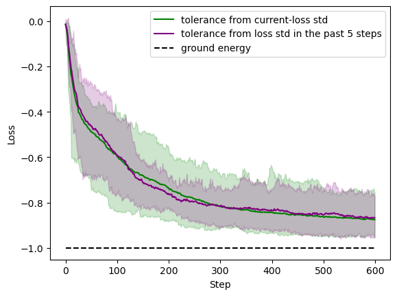
The efficacy of this new tolerance definition is confirmed by reproducing the experiment on QN-SPSA in Fig. 1(b) from reference 1. In the following figure, we show the performance of the optimizer with the two tolerance definitions for an 11-qubit system. The shaded areas are the profiles of 25 trials of the experiment. One can confirm the past-\(N\)-step (\(N=5\) for the plot) standard deviation works just as well. With the new choice of the tolerance, for each step, the QN-SPSA will only need to execute 2 (for gradient) + 4 (for metric tensor) + 2 (for the current and the next-step loss) = 8 circuits. In practice, we measure a 50% reduction in the stepwise optimization time.

The test is done with Amazon Braket Hybrid Jobs, as it is a handy tool to scale up experiments systematically. We will show how to do that towards the end of the tutorial.

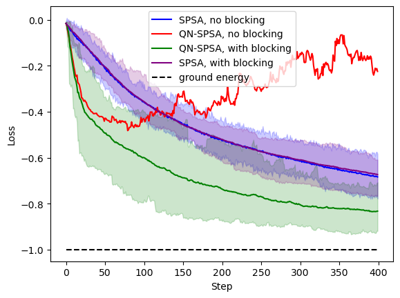
Similarly, with Hybrid Jobs, we can confirm that blocking is necessary for this second-order SPSA optimizer, though it does not make much difference for SPSA. Here, the envelope of the QN-SPSA curves without blocking is not plotted since it is too noisy to visualize. SPSA is implemented by replacing the metric tensor with an identity matrix.

Efficiency improvement

Let’s do a deep dive on how to further improve the execution efficiency of the code. In the code example above, we compute gradient, metric tensor, and the loss values through individual calls on the QNode.__call__() function (in this example, cost_function()). In a handwavy argument, each QNode.__call__() does the following two things: (1) it constructs a tape with the given parameters, and (2) calls qml.execute() to execute the single tape.

However, in this use case, the better practice is to group the tapes and call one qml.execute() on all the tapes. This practice utilizes the batch execution feature from PennyLane, and has a few potential advantages. Some simulators provide parallelization support, so that the grouped tapes can be executed simutaneously. As an example, utilizing the task batching feature from the Braket SV1 simulator, we are able to reduce the optimization time by 75% for large circuits. For quantum hardware, sending tapes in batches could also enable further efficiency improvement in circuit compilation.

With this rewriting, the complete optimizer class is provided in the following cell.

import random
import pennylane as qml
from pennylane import numpy as np
from scipy.linalg import sqrtm
import warnings


class QNSPSA:
    """Quantum natural SPSA optimizer. Refer to https://quantum-journal.org/papers/q-2021-10-20-567/
    for a detailed description of the methodology. When disable_metric_tensor
    is set to be True, the metric tensor estimation is disabled, and QNSPSA is
    reduced to be a SPSA optimizer.

    Args:
        stepsize (float): The learn rate.
        regularization (float): Regularitzation term to the Fubini-Study
            metric tensor for numerical stability.
        finite_diff_step (float): step size to compute the finite difference
            gradient and the Fubini-Study metric tensor.
        resamplings (int): The number of samples to average for each parameter
            update.
        blocking (boolean): When set to be True, the optimizer only accepts
            updates that lead to a loss value no larger than the loss value
            before update, plus a tolerance. The tolerance is set with the
            parameter history_length.
        history_length (int): When blocking is True, the tolerance is set to be
            the average of the cost values in the last history_length steps.
        disable_metric_tensor (boolean): When set to be True, the optimizer is
            reduced to be a (1st-order) SPSA optimizer.
        seed (int): Seed for the random sampling.
    """

    def __init__(
        self,
        stepsize=1e-3,
        regularization=1e-3,
        finite_diff_step=1e-2,
        resamplings=1,
        blocking=True,
        history_length=5,
        disable_metric_tensor=False,
        seed=None,
    ):
        self.stepsize = stepsize
        self.reg = regularization
        self.finite_diff_step = finite_diff_step
        self.metric_tensor = None
        self.k = 1
        self.resamplings = resamplings
        self.blocking = blocking
        self.last_n_steps = np.zeros(history_length)
        self.history_length = history_length
        self.disable_metric_tensor = disable_metric_tensor
        random.seed(seed)
        return

    def step(self, cost, params):
        """Update trainable arguments with one step of the optimizer.

        .. warning::
            When blocking is set to be True, use step_and_cost instead, as loss
            measurements are required for the updates for the case.

        Args:
            cost (qml.QNode): the QNode wrapper for the objective function for
            optimization
            params (np.array): Parameter before update.

        Returns:
            np.array: The new variable values after step-wise update.
        """
        if self.blocking:
            warnings.warn(
                "step_and_cost() instead of step() is called when "
                "blocking is turned on, as the step-wise loss value "
                "is required by the algorithm.",
                stacklevel=2,
            )
            return self.step_and_cost(cost, params)[0]

        if self.disable_metric_tensor:
            return self.__step_core_first_order(cost, params)
        return self.__step_core(cost, params)

    def step_and_cost(self, cost, params):
        """Update trainable parameters with one step of the optimizer and return
        the corresponding objective function value after the step.

        Args:
            cost (qml.QNode): the QNode wrapper for the objective function for
                optimization
            params (np.array): Parameter before update.

        Returns:
            tuple[np.array, float]: the updated parameter and the objective
                function output before the step.
        """
        params_next = (
            self.__step_core_first_order(cost, params)
            if self.disable_metric_tensor
            else self.__step_core(cost, params)
        )

        if not self.blocking:
            loss_curr = cost(params)
            return params_next, loss_curr
        params_next, loss_curr = self.__apply_blocking(cost, params, params_next)
        return params_next, loss_curr

    def __step_core(self, cost, params):
        # Core function that returns the next parameters before applying blocking.
        grad_avg = np.zeros(params.shape)
        tensor_avg = np.zeros((params.size, params.size))
        for i in range(self.resamplings):
            grad_tapes, grad_dir = self.__get_spsa_grad_tapes(cost, params)
            metric_tapes, tensor_dirs = self.__get_tensor_tapes(cost, params)
            raw_results = qml.execute(grad_tapes + metric_tapes, cost.device, None)
            grad = self.__post_process_grad(raw_results[:2], grad_dir)
            metric_tensor = self.__post_process_tensor(raw_results[2:], tensor_dirs)
            grad_avg = grad_avg * i / (i + 1) + grad / (i + 1)
            tensor_avg = tensor_avg * i / (i + 1) + metric_tensor / (i + 1)

        self.__update_tensor(tensor_avg)
        return self.__get_next_params(params, grad_avg)

    def __step_core_first_order(self, cost, params):
        # Reduced core function that returns the next parameters with SPSA rule.
        # Blocking not applied.
        grad_avg = np.zeros(params.shape)
        for i in range(self.resamplings):
            grad_tapes, grad_dir = self.__get_spsa_grad_tapes(cost, params)
            raw_results = qml.execute(grad_tapes, cost.device, None)
            grad = self.__post_process_grad(raw_results, grad_dir)
            grad_avg = grad_avg * i / (i + 1) + grad / (i + 1)
        return params - self.stepsize * grad_avg

    def __post_process_grad(self, grad_raw_results, grad_dir):
        # With the quantum measurement results from the 2 gradient tapes,
        # compute the estimated gradient. Returned gradient is a tensor
        # of the same shape with the input parameter tensor.
        loss_forward, loss_backward = grad_raw_results
        grad = (loss_forward - loss_backward) / (2 * self.finite_diff_step) * grad_dir
        return grad

    def __post_process_tensor(self, tensor_raw_results, tensor_dirs):
        # With the quantum measurement results from the 4 metric tensor tapes,
        # compute the estimated raw metric tensor. Returned raw metric tensor
        # is a tensor of shape (d x d), d being the dimension of the input parameter
        # to the ansatz.
        tensor_finite_diff = (
            tensor_raw_results[0][0]
            - tensor_raw_results[1][0]
            - tensor_raw_results[2][0]
            + tensor_raw_results[3][0]
        )
        metric_tensor = (
            -(
                np.tensordot(tensor_dirs[0], tensor_dirs[1], axes=0)
                + np.tensordot(tensor_dirs[1], tensor_dirs[0], axes=0)
            )
            * tensor_finite_diff
            / (8 * self.finite_diff_step * self.finite_diff_step)
        )
        return metric_tensor

    def __get_next_params(self, params, gradient):
        grad_vec, params_vec = gradient.reshape(-1), params.reshape(-1)
        new_params_vec = np.linalg.solve(
            self.metric_tensor,
            (-self.stepsize * grad_vec + np.matmul(self.metric_tensor, params_vec)),
        )
        return new_params_vec.reshape(params.shape)

    def __get_perturbation_direction(self, params):
        param_number = len(params) if isinstance(params, list) else params.size
        sample_list = random.choices([-1, 1], k=param_number)
        direction = np.array(sample_list).reshape(params.shape)
        return direction

    def __get_spsa_grad_tapes(self, cost, params):
        # Returns the 2 tapes along with the sampled direction that will be
        # used to estimate the gradient per optimization step. The sampled
        # direction is of the shape of the input parameter.
        direction = self.__get_perturbation_direction(params)
        cost.construct([params + self.finite_diff_step * direction], {})
        tape_forward = cost.tape.copy(copy_operations=True)
        cost.construct([params - self.finite_diff_step * direction], {})
        tape_backward = cost.tape.copy(copy_operations=True)
        return [tape_forward, tape_backward], direction

    def __update_tensor(self, tensor_raw):
        tensor_avg = self.__get_tensor_moving_avg(tensor_raw)
        tensor_regularized = self.__regularize_tensor(tensor_avg)
        self.metric_tensor = tensor_regularized
        self.k += 1

    def __get_tensor_tapes(self, cost, params):
        # Returns the 4 tapes along with the 2 sampled directions that will be
        # used to estimate the raw metric tensor per optimization step. The sampled
        # directions are 1d vectors of the length of the input parameter dimension.
        dir1 = self.__get_perturbation_direction(params)
        dir2 = self.__get_perturbation_direction(params)
        perturb1 = dir1 * self.finite_diff_step
        perturb2 = dir2 * self.finite_diff_step
        dir_vecs = dir1.reshape(-1), dir2.reshape(-1)

        tapes = [
            self.__get_overlap_tape(cost, params, params + perturb1 + perturb2),
            self.__get_overlap_tape(cost, params, params + perturb1),
            self.__get_overlap_tape(cost, params, params - perturb1 + perturb2),
            self.__get_overlap_tape(cost, params, params - perturb1),
        ]
        return tapes, dir_vecs

    def __get_overlap_tape(self, cost, params1, params2):
        op_forward = self.__get_operations(cost, params1)
        op_inv = self.__get_operations(cost, params2)

        with qml.tape.QuantumTape() as tape:
            for op in op_forward:
                qml.apply(op)
            for op in reversed(op_inv):
                op.adjoint()
            qml.probs(wires=cost.tape.wires.labels)
        return tape

    def __get_operations(self, cost, params):
        # Given a QNode, returns the list of operations before the measurement.
        cost.construct([params], {})
        return cost.tape.operations

    def __get_tensor_moving_avg(self, metric_tensor):
        # For numerical stability: averaging on the Fubini-Study metric tensor.
        if self.metric_tensor is None:
            self.metric_tensor = np.identity(metric_tensor.shape[0])
        return self.k / (self.k + 1) * self.metric_tensor + 1 / (self.k + 1) * metric_tensor

    def __regularize_tensor(self, metric_tensor):
        # For numerical stability: Fubini-Study metric tensor regularization.
        tensor_reg = np.real(sqrtm(np.matmul(metric_tensor, metric_tensor)))
        return (tensor_reg + self.reg * np.identity(metric_tensor.shape[0])) / (1 + self.reg)

    def __apply_blocking(self, cost, params_curr, params_next):
        # For numerical stability: apply the blocking condition on the parameter update.
        cost.construct([params_curr], {})
        tape_loss_curr = cost.tape.copy(copy_operations=True)
        cost.construct([params_next], {})
        tape_loss_next = cost.tape.copy(copy_operations=True)

        loss_curr, loss_next = qml.execute([tape_loss_curr, tape_loss_next], cost.device, None)
        # self.k has been updated earlier.
        ind = (self.k - 2) % self.history_length
        self.last_n_steps[ind] = loss_curr

        tol = (
            2 * self.last_n_steps.std()
            if self.k > self.history_length
            else 2 * self.last_n_steps[: self.k - 1].std()
        )

        if loss_curr + tol < loss_next:
            params_next = params_curr
        return params_next, loss_curr

Let’s see how it performs on our QAOA example:

opt = QNSPSA(stepsize=5e-2)
params_init = 2 * np.pi * (np.random.rand(2, depth) - 0.5)
params = params_init
for i in range(300):
    params, loss = opt.step_and_cost(cost_function, params)
    if i % 40 == 0:
        print(f"Step {i}: cost = {loss:.4f}")

Out:

Step 0: cost = -2.0730
Step 40: cost = -2.5390
Step 80: cost = -2.7240
Step 120: cost = -2.6760
Step 160: cost = -2.7540
Step 200: cost = -2.7060
Step 240: cost = -2.8110
Step 280: cost = -2.7930

The optimizer performs reasonably well: the loss drops over optimization steps and converges finally. We then reproduce the benchmarking test between the gradient descent, quantum natural gradient descent, SPSA and QN-SPSA in Fig. 1(b) of reference 1 with the following job. You can find a more detailed version of the example in this notebook, with its dependencies in the source_scripts folder.

Note

In order for the remainder of this demo to work, you will need to have done 3 things:

1. Copied the source_scripts folder (linked above) to your working directory

2. Authenticated with AWS locally

3. Granted yourself the appropriate permissions as described in this AWS Braket setup document

from braket.aws import AwsSession, AwsQuantumJob
from braket.jobs.config import InstanceConfig
from braket.jobs.image_uris import Framework, retrieve_image
import boto3

region_name = AwsSession().region
image_uri = retrieve_image(Framework.BASE, region_name)

n_qubits = 11

hyperparameters = {
    "n_qubits": n_qubits,
    "n_layers": 4,
    "shots": 8192,
    "max_iter": 600,
    "learn_rate": 1e-2,
    "spsa_repeats": 25,
}

job_name = f"ref-paper-benchmark-qubit-{n_qubits}"
instance_config = InstanceConfig(instanceType="ml.m5.large", volumeSizeInGb=30, instanceCount=1)

job = AwsQuantumJob.create(
    device="local:pennylane/lightning.qubit",
    source_module="source_scripts",
    entry_point="source_scripts.benchmark_ref_paper_converge_speed",
    job_name=job_name,
    hyperparameters=hyperparameters,
    instance_config=instance_config,
    image_uri=image_uri,
    wait_until_complete=False,
)

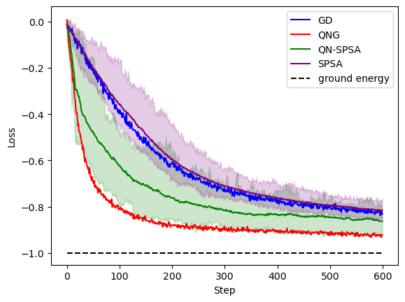
Visualizing the job results, we get the following plot. The results are well aligned with the observations from Gacon et al. 1. The stepwise optimization times for GD, QNG, SPSA and QN-SPSA are measured to be 0.43s, 0.75s, 0.03s and 0.20s. In this example, the average behavior of SPSA matches the one from GD. QNG performs the best among the 4 candidates, but it requires the most circuit executions and shots per step. In particular, for QPUs, this is a severe disadvantage of this method. From the more shot-frugal options, QN-SPSA demonstrates the fastest convergence and best final accuracy, making it a promising candidate for variational algorithms.

To sum up, in this tutorial, we showed step-by-step how we can implement the QN-SPSA optimizer with PennyLane, along with a few tricks to further improve the optimizer’s performance. We also demonstrated how one can scale up the benchmarking experiments with Amazon Braket Hybrid Jobs.

References

1(1,2,3,4,5,6)

Gacon, J., Zoufal, C., Carleo, G., & Woerner, S. (2021). Simultaneous perturbation stochastic approximation of the quantum fisher information. Quantum, 5, 567.

2

Simultaneous perturbation stochastic approximation (2022). Wikipedia. https://en.wikipedia.org/wiki/Simultaneous_perturbation_stochastic_approximation

3(1,2)

Stokes, J., Izaac, J., Killoran, N., & Carleo, G. (2020). Quantum natural gradient. Quantum, 4, 269.

4

Fubini–Study metric (2022). Wikipedia. https://en.wikipedia.org/wiki/Fubini%E2%80%93Study_metric

5

Yamamoto, N. (2019). On the natural gradient for variational quantum eigensolver. arXiv preprint arXiv:1909.05074.

6(1,2)

Spall, J. C. (1997). Accelerated second-order stochastic optimization using only function measurements. In Proceedings of the 36th IEEE Conference on Decision and Control (Vol. 2, pp. 1417-1424). IEEE.

About the author

Yiheng Duan

Yiheng is an Applied Scientist at AWS Braket. Yiheng works at the intersection of quantum computing and machine learning and can be reached via yiheng@amazon.com.

demos/qnspsa

 

Download Python script

 

Download Notebook

 

View on GitHub