Variationally optimizing measurement protocols

Author: Johannes Jakob Meyer — Posted: 18 June 2020. Last updated: 18 November 2021.

In this tutorial we use the variational quantum algorithm from Ref. 1 to optimize a quantum sensing protocol.

Background

Quantum technologies are a rapidly expanding field with applications ranging from quantum computers to quantum communication lines. In this tutorial, we study a particular application of quantum technologies, namely Quantum Metrology. It exploits quantum effects to enhance the precision of measurements. One of the most impressive examples of a successful application of quantum metrology is gravitational wave interferometers like LIGO that harness non-classical light to increase the sensitivity to passing gravitational waves.

A quantum metrological experiment, which we call a protocol, can be modelled in the following way. As a first step, a quantum state \(\rho_0\) is prepared. This state then undergoes a possibly noisy quantum evolution that depends on a vector of parameters \(\boldsymbol{\phi}\) we are interested in—we say the quantum evolution encodes the parameters. The values \(\boldsymbol{\phi}\) can for example be a set of phases that are picked up in an interferometer. As we use the quantum state to probe the encoding evolution, we will call it the probe state.

After the parameters are encoded, we have a new state \(\rho(\boldsymbol{\phi})\) which we then need to measure. We can describe any possible measurement in quantum mechanics using a positive operator-valued measurement consisting of a set of operators \(\{ \Pi_l \}\). Measuring those operators gives us the output probabilities

\[p_l(\boldsymbol{\phi}) = \langle \Pi_l \rangle = \operatorname{Tr}(\rho(\boldsymbol{\phi}) \Pi_l).\]

As the last step of our protocol, we have to estimate the parameters \(\boldsymbol{\phi}\) from these probabilities, e.g., through maximum likelihood estimation. Intuitively, we will get the best precision in doing so if the probe state is most “susceptible” to the encoding evolution and the corresponding measurement can distinguish the states for different values of \(\boldsymbol{\phi}\) well.

The variational algorithm

We now introduce a variational algorithm to optimize such a sensing protocol. As a first step, we parametrize both the probe state \(\rho_0 = \rho_0(\boldsymbol{\theta})\) and the POVM \(\Pi_l = \Pi_l(\boldsymbol{\mu})\) using suitable quantum circuits with parameters \(\boldsymbol{\theta}\) and \(\boldsymbol{\mu}\) respectively. The parameters should now be adjusted in a way that improves the sensing protocol, and to quantify this, we need a suitable cost function.

Luckily, there exists a mathematical tool to quantify the best achievable estimation precision, the Cramér-Rao bound. Any estimator \(\mathbb{E}(\hat{\boldsymbol{\varphi}}) = \boldsymbol{\phi}\) we could construct fulfills the following condition on its covariance matrix which gives a measure of the precision of the estimation:

\[\operatorname{Cov}(\hat{\boldsymbol{\varphi}}) \geq \frac{1}{n} I^{-1}_{\boldsymbol{\phi}},\]

where \(n\) is the number of samples and \(I_{\boldsymbol{\phi}}\) is the Classical Fisher Information Matrix with respect to the entries of \(\boldsymbol{\phi}\). It is defined as

\[[I_{\boldsymbol{\phi}}]_{jk} := \sum_l \frac{(\partial_j p_l)(\partial_k p_l)}{p_l},\]

where we used \(\partial_j\) as a shorthand notation for \(\frac{\partial}{\partial \phi_j}\). The Cramér-Rao bound has the very powerful property that it can always be saturated in the limit of many samples! This means we are guaranteed that we can construct a “best estimator” for the vector of parameters.

This in turn means that the right hand side of the Cramér-Rao bound would make for a great cost function. There is only one remaining problem, namely that it is matrix-valued, but we need a scalar cost function. To obtain such a scalar quantity, we multiply both sides of the inequality with a positive-semidefinite weighting matrix \(W\) and then perform a trace,

\[\operatorname{Tr}(W\operatorname{Cov}(\hat{\boldsymbol{\varphi}})) \geq \frac{1}{n} \operatorname{Tr}(W I^{-1}_{\boldsymbol{\phi}}).\]

As its name suggests, \(W\) can be used to weight the importance of the different entries of \(\boldsymbol{\phi}\). The right-hand side is now a scalar quantifying the best attainable weighted precision and can be readily used as a cost function:

\[C_W(\boldsymbol{\theta}, \boldsymbol{\mu}) = \operatorname{Tr}(W I^{-1}_{\boldsymbol{\phi}}(\boldsymbol{\theta}, \boldsymbol{\mu})).\]

With the cost function in place, we can use Pennylane to optimize the variational parameters \(\boldsymbol{\theta}\) and \(\boldsymbol{\mu}\) to obtain a good sensing protocol. The whole pipeline is depicted below:

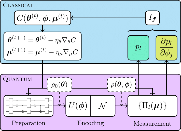
Here, the encoding process is modeled as a unitary evolution \(U(\boldsymbol{\phi})\) followed by a parameter-independent noise channel \(\mathcal{N}\).

Ramsey spectroscopy

In this demonstration, we will study Ramsey spectroscopy, a widely used technique for quantum metrology with atoms and ions. The encoded parameters are phase shifts \(\boldsymbol{\phi}\) arising from the interaction of probe ions modeled as two-level systems with an external driving force. We represent the noise in the parameter encoding using a phase damping channel (also known as dephasing channel) with damping constant \(\gamma\). We consider a pure probe state on three qubits and a projective measurement, where the computational basis is parametrized by local unitaries.

The above method is actually not limited to the estimation of the parameters \(\boldsymbol{\phi}\), but can also be used to optimize estimators for functions of those parameters! To add this interesting aspect to the tutorial, we will seek an optimal protocol for the estimation of the Fourier amplitudes of the phases:

\[f_j(\boldsymbol{\boldsymbol{\phi}}) = \left|\sum_k \phi_k \mathrm{e}^{-i j k \frac{2\pi}{N}}\right|^2.\]

For three phases, there are two independent amplitudes \(f_0\) and \(f_1\). To include the effect of the function, we need to replace the classical Fisher information matrix with respect to \(\boldsymbol{\phi}\) with the Fisher information matrix with respect to the entries \(f_0\) and \(f_1\). To this end we can make use of the following identity which relates the two matrices:

\[I_{\boldsymbol{f}} = J^T I_{\boldsymbol{\phi}} J,\]

where \(J_{kl} = \frac{\partial f_k}{\partial \phi_l}\) is the Jacobian of \(\boldsymbol{f}\).

We now turn to the actual implementation of the scheme.

import pennylane as qml
from pennylane import numpy as np

Modeling the sensing process

We will first specify the device to carry out the simulations. As we want to model a noisy system, it needs to be capable of mixed-state simulations. We will choose the cirq.mixedsimulator device from the Pennylane-Cirq plugin for this tutorial.

dev = qml.device("cirq.mixedsimulator", wires=3, shots=1000)

Next, we model the parameter encoding. The phase shifts are recreated using the Pauli Z rotation gate. The phase-damping noise channel is available as a custom Cirq gate.

from pennylane_cirq import ops as cirq_ops


def encoding(phi, gamma):
    for i in range(3):
        qml.RZ(phi[i], wires=[i])
        cirq_ops.PhaseDamp(gamma, wires=[i])

We now choose a parametrization for both the probe state and the POVM. To be able to parametrize all possible probe states and all local measurements, we make use of the ArbitraryStatePreparation template from PennyLane.

def ansatz(weights):
    qml.ArbitraryStatePreparation(weights, wires=[0, 1, 2])

NUM_ANSATZ_PARAMETERS = 14

def measurement(weights):
    for i in range(3):
        qml.ArbitraryStatePreparation(
            weights[2 * i : 2 * (i + 1)], wires=[i]
        )

NUM_MEASUREMENT_PARAMETERS = 6

We now have everything at hand to model the quantum part of our experiment as a QNode. We will return the output probabilities necessary to compute the Classical Fisher Information Matrix.

@qml.qnode(dev)
def experiment(weights, phi, gamma=0.0):
    ansatz(weights[:NUM_ANSATZ_PARAMETERS])
    encoding(phi, gamma)
    measurement(weights[NUM_ANSATZ_PARAMETERS:])

    return qml.probs(wires=[0, 1, 2])

# Draw the circuit at the given parameter values
print(qml.draw(experiment, expansion_strategy='device')(
    np.arange(NUM_ANSATZ_PARAMETERS + NUM_MEASUREMENT_PARAMETERS),
    np.zeros(3),
    gamma=0.2)
)

Out:

0: ──H──RZ(0.00)──H──RX(1.57)──RZ(1.00)──RX(-1.57)──H─────────────────────────────────────────────
1: ──H──RZ(2.00)──H──RX(1.57)──RZ(3.00)──RX(-1.57)──H─╭X──RZ(6.00)─╭X──H──H────────╭X──RZ(7.00)─╭X
2: ──H──RZ(4.00)──H──RX(1.57)──RZ(5.00)──RX(-1.57)──H─╰●───────────╰●──H──RX(1.57)─╰●───────────╰●

────────────────╭X──RZ(8.00)─╭X──H──H────────╭X──RZ(9.00)─╭X──H──────────H─╭X──RZ(10.00)─╭X──H
───H──────────H─╰●───────────╰●──H──RX(1.57)─╰●───────────╰●──RX(-1.57)────│─────────────│────
───RX(-1.57)──H────────────────────────────────────────────────────────────╰●────────────╰●──H

───H────────╭X──RZ(11.00)─╭X──H──────────H────╭X──RZ(12.00)─╭X──H──H──────────────╭X──RZ(13.00)─╭X
────────────│─────────────│───H────────────╭X─╰●────────────╰●─╭X──H──H────────╭X─╰●────────────╰●
───RX(1.57)─╰●────────────╰●──RX(-1.57)──H─╰●──────────────────╰●──H──RX(1.57)─╰●─────────────────

───H──RZ(0.00)───PhaseDamp(0.20)──H────────────────RZ(14.00)──H──────────RX(1.57)──RZ(15.00)
──╭X──H──────────RZ(0.00)─────────PhaseDamp(0.20)──H──────────RZ(16.00)──H─────────RX(1.57)─
──╰●──RX(-1.57)──RZ(0.00)─────────PhaseDamp(0.20)──H──────────RZ(18.00)──H─────────RX(1.57)─

───RX(-1.57)────────────┤ ╭Probs
───RZ(17.00)──RX(-1.57)─┤ ├Probs
───RZ(19.00)──RX(-1.57)─┤ ╰Probs

Evaluating the cost function

Now, let’s turn to the cost function itself. The most important ingredient is the Classical Fisher Information Matrix, which we compute using a separate function that uses the explicit parameter-shift rule to enable differentiation.

def CFIM(weights, phi, gamma):
    p = experiment(weights, phi, gamma=gamma)
    dp = []

    for idx in range(3):
        # We use the parameter-shift rule explicitly
        # to compute the derivatives
        shift = np.zeros_like(phi)
        shift[idx] = np.pi / 2

        plus = experiment(weights, phi + shift, gamma=gamma)
        minus = experiment(weights, phi - shift, gamma=gamma)

        dp.append(0.5 * (plus - minus))

    matrix = [0] * 9
    for i in range(3):
        for j in range(3):
            matrix[3 * i + j] = np.sum(dp[i] * dp[j] / p)

    return np.array(matrix).reshape((3, 3))

As the cost function contains an inversion, we add a small regularization to it to avoid inverting a singular matrix. As additional parameters, we add the weighting matrix \(W\) and the Jacobian \(J\).

def cost(weights, phi, gamma, J, W, epsilon=1e-10):
    return np.trace(
        W
        @ np.linalg.inv(
            J.T @ CFIM(weights, phi, gamma) @ J + np.eye(2) * epsilon
        )
    )

To compute the Jacobian, we make use of sympy. The two independent Fourier amplitudes are computed using the discrete Fourier transform matrix \(\Omega_{jk} = \frac{\omega^{jk}}{\sqrt{N}}\) with \(\omega = \exp(-i \frac{2\pi}{N})\).

import sympy
import cmath

# Prepare symbolic variables
x, y, z = sympy.symbols("x y z", real=True)
phi = sympy.Matrix([x, y, z])

# Construct discrete Fourier transform matrix
omega = sympy.exp((-1j * 2.0 * cmath.pi) / 3)
Omega = sympy.Matrix([[1, 1, 1], [1, omega ** 1, omega ** 2]]) / sympy.sqrt(3)

# Compute Jacobian
jacobian = (
    sympy.Matrix(list(map(lambda x: abs(x) ** 2, Omega @ phi))).jacobian(phi).T
)
# Lambdify converts the symbolic expression to a python function
jacobian = sympy.lambdify((x, y, z), sympy.re(jacobian))

Optimizing the protocol

We can now turn to the optimization of the protocol. We will fix the dephasing constant at \(\gamma=0.2\) and the ground truth of the sensing parameters at \(\boldsymbol{\phi} = (1.1, 0.7, -0.6)\) and use an equal weighting of the two Fourier amplitudes, corresponding to \(W = \mathbb{I}_2\).

gamma = 0.2
phi = np.array([1.1, 0.7, -0.6])
J = jacobian(*phi)
W = np.eye(2)

We are now ready to perform the optimization. We will initialize the weights at random. Then we make use of the Adagrad optimizer. Adaptive gradient descent methods are advantageous as the optimization of quantum sensing protocols is very sensitive to the step size.

def opt_cost(weights, phi=phi, gamma=gamma, J=J, W=W):
    return cost(weights, phi, gamma, J, W)


# Seed for reproducible results
np.random.seed(395)
weights = np.random.uniform(
    0, 2 * np.pi, NUM_ANSATZ_PARAMETERS + NUM_MEASUREMENT_PARAMETERS, requires_grad=True
)

opt = qml.AdagradOptimizer(stepsize=0.1)

print("Initialization: Cost = {:6.4f}".format(opt_cost(weights)))
for i in range(20):
    weights, cost_ = opt.step_and_cost(opt_cost, weights)

    if (i + 1) % 5 == 0:
        print(
            "Iteration {:>4}: Cost = {:6.4f}".format(i + 1, cost_)
        )

Out:

Initialization: Cost = 4.1074
Iteration    5: Cost = 2.0604
Iteration   10: Cost = 1.8455
Iteration   15: Cost = 1.7749
Iteration   20: Cost = 1.5183

Comparison with the standard protocol

Now we want to see how our protocol compares to the standard Ramsey interferometry protocol. The probe state in this case is a tensor product of three separate \(|+\rangle\) states while the encoded state is measured in the \(|+\rangle / |-\rangle\) basis. We can recreate the standard schemes with specific weights for our setup.

Ramsey_weights = np.zeros_like(weights)
Ramsey_weights[1:6:2] = np.pi / 2
Ramsey_weights[15:20:2] = np.pi / 2
print(
    "Cost for standard Ramsey sensing = {:6.4f}".format(
        opt_cost(Ramsey_weights)
    )
)

Out:

Cost for standard Ramsey sensing = 1.7394

We can now make a plot to compare the noise scaling of the above probes.

gammas = np.linspace(0, 0.75, 21)
comparison_costs = {
    "optimized": [],
    "standard": [],
}

for gamma in gammas:
    comparison_costs["optimized"].append(
        cost(weights, phi, gamma, J, W)
    )
    comparison_costs["standard"].append(
        cost(Ramsey_weights, phi, gamma, J, W)
    )

import matplotlib.pyplot as plt

plt.semilogy(gammas, comparison_costs["optimized"], label="Optimized")
plt.semilogy(gammas, comparison_costs["standard"], label="Standard")
plt.xlabel(r"$\gamma$")
plt.ylabel("Weighted Cramér-Rao bound")
plt.legend()
plt.grid()
plt.show()

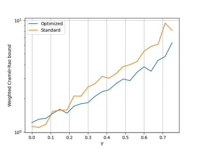
We see that after only 20 gradient steps, we already found a sensing protocol that has a better noise resilience than standard Ramsey spectroscopy!

This tutorial shows that variational methods are useful for quantum metrology. The are numerous avenues open for further research: one could study more intricate sensing problems, different noise models, and other platforms like optical systems.

For more intricate noise models that can’t be realized on quantum hardware, Ref. 1 offers a way to move certain parts of the algorithm to the classical side. It also provides extensions of the method to include prior knowledge about the distribution of the underlying parameters or to factor in mutual time-dependence of parameters and encoding noise.

References

1(1,2)

Johannes Jakob Meyer, Johannes Borregaard, Jens Eisert. “A variational toolbox for quantum multi-parameter estimation.” arXiv:2006.06303, 2020.

About the author

Johannes Jakob Meyer

Johannes Jakob is a PhD student in Jens Eisert's group at the FU Berlin. He strives to establish hard facts about near-term quantum devices and convert those into useful applications. His personal website is website johannesjakobmeyer.com.

demos/tutorial_quantum_metrology

 

Download Python script

 

Download Notebook

 

View on GitHub