Quantum Circuit Cutting

Authors: Gideon Uchehara, Matija Medvidović, Anuj Apte — Posted: 02 September 2022. Last updated: 02 September 2022.

Introduction

Quantum circuits with a large number of qubits are difficult to simulate. They cannot be programmed on actual hardware due to size constraints (insufficient qubits), and they are also error-prone. What if we “cut” a large circuit into smaller, more manageable pieces? This is the main idea behind the algorithm that allows you to simulate large quantum circuits on a small quantum computer called quantum circuit cutting.

In this demo, we will first introduce the theory behind quantum circuit cutting based on Pauli measurements and see how it is implemented in PennyLane. This method was first introduced in 1. Thereafter, we discuss the theoretical basis on randomized circuit cutting with two-designs and demonstrate the resulting improvement in performance compared to Pauli measurement based circuit cutting for an instance of Quantum Approximate Optimization Algorithm (QAOA).

Background: Understanding the Pauli cutting method

Consider a two-level quantum system in an arbitrary state, described by density matrix \(\rho\). The quantum state \(\rho\) can be expressed as a linear combination of the Pauli matrices:

\[\rho = \frac{1}{2}\sum_{i=1}^{8} c_i Tr(\rho O_i)\rho_i.\]

Here, we have denoted Pauli matrices by \(O_i\), their eigenprojectors by \(\rho_i\) and their corresponding eigenvalues by \(c_i\). In the above equation,

\[O_1 = O_2 = I,\]

\[O_3 = O_4 = X,\]

\[O_5 = O_6 = Y\]

and

\[O_7 = O_8 = Z.\]

Also,

\[\rho_1 = \rho_7=\left | {0} \right\rangle \left\langle {0} \right |,\]

\[\rho_2 = \rho_8 = \left | {1} \right\rangle \left\langle {1} \right |,\]

\[\rho_3 = \left | {+} \right\rangle \left\langle {+} \right |,\]

\[\rho_4 = \left | {-} \right\rangle \left\langle {-} \right |,\]

\[\rho_5 = \left | {+i} \right\rangle \left\langle {+i} \right |,\]

\[\rho_6 = \left | {-i} \right\rangle \left\langle {-i} \right |\]

and

\[c_i = \pm 1.\]

The above equation can be implemented as a quantum circuit on a quantum computer. To do this, each term \(Tr(\rho O_i)\rho_i\) in the equation is broken into two parts. The first part, \(Tr(\rho O_i)\) is the expectation of the observable \(O_i\) when the system is in the state \(\rho\). Let’s call this first circuit subcircuit-\(u\). The second part, \(\rho_i\) is initialization or preparation of the eigenstate, \(\rho_i\). Let’s call this Second circuit subcircuit-\(v\). The above equation shows how we can recover a quantum state after a is cut made on one of its qubits as shown in figure 1. This forms the core of quantum circuit cutting.

It turns out that we only have to do three measurements \(\left (Tr(\rho X), Tr(\rho Y), Tr(\rho Z) \right)\) for subcircuit-\(u\) and initialize subcircuit-\(v\) with only four states: \(\left | {0} \right\rangle\), \(\left | {1} \right\rangle\), \(\left | {+} \right\rangle\) and \(\left | {+i} \right\rangle\). The other two nontrivial expectation values for states \(\left | {-} \right\rangle\) and \(\left | {- i} \right\rangle\) can be derived with classical post-processing.

In general, there is a resolution of the identity along a wire (qubit) that we can interpret as circuit cutting. In the following section, we will provide a more clever way of resolving the same identity that leads to fewer shots needed to estimate observables.

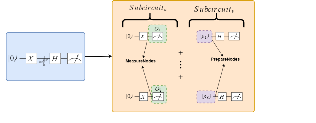
Figure 1. The Pauli circuit cutting method for 1-qubit circuit. The first half of the cut circuit on the left (subcircuit-u) is the part with MeasureNode. The second half of the cut circuit on the right (subcircuit-v) is the part with PrepareNode

PennyLane implementation

PennyLane’s built-in circuit cutting algorithm, qml.cut_circuit, takes a large quantum circuit and decomposes it into smaller subcircuits that are executed on a small quantum device. The results from executing the smaller subcircuits are then recombined through some classical post-processing to obtain the original result of the large quantum circuit.

Let’s simulate a “real-world” scenario with qml.cut_circuit using the circuit below.

# Import the relevant libraries
import pennylane as qml
from pennylane import numpy as np

dev = qml.device("default.qubit", wires=3)


@qml.qnode(dev)
def circuit(x):
    qml.RX(x, wires=0)
    qml.RY(0.9, wires=1)
    qml.RX(0.3, wires=2)

    qml.CZ(wires=[0, 1])
    qml.RY(-0.4, wires=0)

    qml.CZ(wires=[1, 2])

    return qml.expval(qml.pauli.string_to_pauli_word("ZZZ"))


x = np.array(0.531, requires_grad=True)
fig, ax = qml.draw_mpl(circuit)(x)

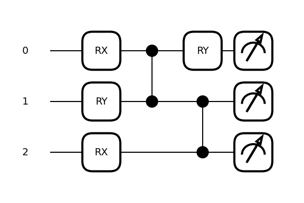
Given the above quantum circuit, our goal is to simulate a 3-qubit quantum circuit on a 2-qubit quantum computer. This means that we have to cut the circuit such that the resulting subcircuits have at most 2 qubits.

Apart from ensuring that the number of qubits for each subcircuit does not exceed the number of qubits on our quantum device, we also have to ensure that the resulting subcircuits have the most efficient classical post-processing. This is not quite trivial to determine in most cases, but for the above circuit, the best cut location turns out to be between the two CZ gates on qubit 1 (more on this later). Hence, we place a WireCut operation at that location as shown below:

dev = qml.device("default.qubit", wires=3)

# Quantum Circuit with QNode


@qml.qnode(dev)
def circuit(x):
    qml.RX(x, wires=0)
    qml.RY(0.9, wires=1)
    qml.RX(0.3, wires=2)

    qml.CZ(wires=[0, 1])
    qml.RY(-0.4, wires=0)

    qml.WireCut(wires=1)  # Cut location

    qml.CZ(wires=[1, 2])

    return qml.expval(qml.pauli.string_to_pauli_word("ZZZ"))


x = np.array(0.531, requires_grad=True)  # Defining the parameter x
fig, ax = qml.draw_mpl(circuit)(x)  # Drawing circuit

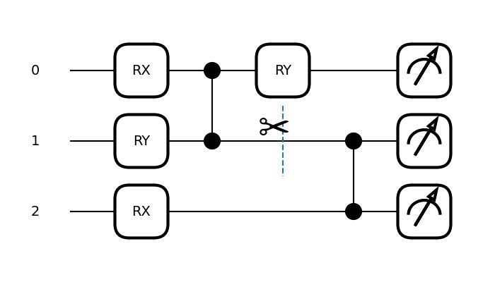
The double vertical lines between the two CZ gates on qubit 1 in the above figure show where we have chosen to cut. This is where the WireCut operation is inserted. WireCut is used to manually mark locations for wire cuts.

Next, we apply qml.cut_circuit operation as a decorator to the circuit function to perform circuit cutting on the quantum circuit.

dev = qml.device("default.qubit", wires=3)

# Quantum Circuit with QNode


@qml.cut_circuit()  # Applying qml.cut_circuit for circuit cut operation
@qml.qnode(dev)
def circuit(x):
    qml.RX(x, wires=0)
    qml.RY(0.9, wires=1)
    qml.RX(0.3, wires=2)

    qml.CZ(wires=[0, 1])
    qml.RY(-0.4, wires=0)

    qml.WireCut(wires=1)  # Cut location

    qml.CZ(wires=[1, 2])

    return qml.expval(qml.pauli.string_to_pauli_word("ZZZ"))


x = np.array(0.531, requires_grad=True)
circuit(x)  # Executing the quantum circuit

Out:

0.47165198882111176

Let’s explore what happens behind the scenes in qml.cut_circuit. When the circuit qnode function is executed, the quantum circuit is converted to a quantum tape and then to a graph. Any WireCut in the quantum circuit graph is replaced with MeasureNode and PrepareNode pairs as shown in figure 2. The MeasureNode is the point on the cut qubit that indicates where to measure the observable \(O_i\) after cut. On the other hand, the PrepareNode is the point on the cut qubit that indicates Where to initialize the state \(\rho\) after cut. Both MeasureNode and PrepareNode are placeholder operations that allow us to cut the quantum circuit graph and then iterate over measurements of Pauli observables and preparations of their corresponding eigenstates configurations at cut locations.

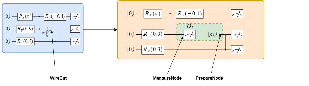
Figure 2. Replace WireCut with MeasureNode and PrepareNode

Cutting at the said location gives two graph fragments with 2 qubits each. To separate these fragments into different subcircuit graphs, the fragment_graph() function is called to pull apart the quantum circuit graph as shown in figure 3. The subcircuit graphs are reconverted back to quantum tapes and qml.cut_circuit runs multiple configurations of the 2-qubit subcircuit tapes which are then post-processed to replicate the result of the uncut circuit.

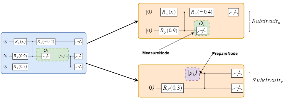
Figure 3. Separate fragments into different subcircuits

Automatic cut placement

We manually found a good cut position, but what if we didn’t know where it was in general? Changing cut positions results in different outcomes in terms of simulation efficiency, so choosing the optimal cut reduces post-processing overhead and improves simulation efficiency.

Automatic cut placment is a PennyLane functionality that aids us in finding the optimal cut that fragments a circuit such that the classical post-processing overhead is minimized. The main algorithm behind automatic cut placement is graph partitioning

If auto_cutter is enabled in qml.cut_circuit, PennyLane makes attempts to find an optimal cut using graph partitioning. Whenever it is difficult to manually determine the optimal cut location, this is the recommended approach to circuit cutting. The following example shows this capability on the same circuit as above but with the WireCut removed.

dev = qml.device("default.qubit", wires=3)


@qml.cut_circuit(auto_cutter=True)  # auto_cutter enabled
@qml.qnode(dev)
def circuit(x):
    qml.RX(x, wires=0)
    qml.RY(0.9, wires=1)
    qml.RX(0.3, wires=2)

    qml.CZ(wires=[0, 1])
    qml.RY(-0.4, wires=0)

    qml.CZ(wires=[1, 2])

    return qml.expval(qml.pauli.string_to_pauli_word("ZZZ"))


x = np.array(0.531, requires_grad=True)
circuit(x)

Out:

0.47165198882111176

Randomized Circuit Cutting

After reviewing the standard circuit cutting based on Pauli measurements on single qubits, we are now ready to discuss an improved circuit cutting protocol that uses randomized measurements to speed up circuit cutting. Our description of this method will be based on the recently published work 2.

The key idea behind this approach is to use measurements in an entagled basis that is based on a unitary 2-design to get more information about the state with fewer measurements compared to single qubit Pauli measurements.

The concept of 2-designs is simple — a unitary 2-design is finite collection of unitaries such that the average of any degree 2 polynomial function of a linear operator over the design is exactly the same as the average over Haar random measure. For further explanation of this measure read the Haar Measure demo.

More precisely, let \(P(U)\) be a polynomial with homogeneous degree at most two in the entries of a unitary matrix \(U\), and degree two in the complex conjugates of those entries. A unitary 2-design is a set of \(L\) unitaries \(\{U_{L}\}\) such that

\[\frac{1}{L} \sum_{l=1}^{L} P(U_l) = \int_{\mathcal{U}(d)} P (U) d\mu(U)~.\]

The elemements of the Clifford group over the qubits being cut are an example of a 2-design. We don’t have a lot of space here to go into too many details. But fear not - there is an entire demo dedicated to this wonderful topic!

Figure 4. Illustration of Randomized Circuit Cutting based on Two-Designs. Taken from 2.

If \(k\) qubits are being cut, then the dimensionality of the Hilbert space is \(d=2^{k}\). The key idea of Randomized Circuit Cutting is to employ two different quantum channels with probabilities such that together they comprise a resolution of Identity. In the randomized measurement circuit cutting procedure, we trace out the \(k\) qubits and prepare a random basis state with probability \(d/(2d+1)\). For a linear operator \(X \in \mathbf{L}(\mathbb{C}^{d})\) acting on the \(k\) qubits, this operation corresponds to the completely depolarizing channel

\[\Psi_{1}(X) = \textrm{Tr}(X)\frac{\mathbf{1}}{d}~.\]

Otherwise, we perform measure-and-prepare protocol based on a unitary 2-design (e.g. a random Clifford) with probability \((d+1)/(2d+1)\), corresponding to the channel

\[\Psi_{0}(X) = \frac{1}{d+1}\left(\textrm{Tr}(X)\mathbf{1} + X\right)~.\]

The sets of Kraus operators for the channels \(\Psi_{1} and \Psi_{0}\) are

\[\Psi_{1}(X) \xrightarrow{} \left\{ \frac{|i\rangle \langle j|}{\sqrt{d}} \right\} \quad \Psi_{0}(X) \xrightarrow{} \left\{ \frac{\mathbf{1}}{\sqrt{d+1}} ~,~ \frac{|i\rangle \langle j|}{\sqrt{d+1}} \right\}~,\]

where indices \(i,j\) run over the \(d\) basis elements.

Together, these two channels can be used to obtain a resolution of the Identity channel on the \(k\)-qubits as follows

\[X = (d+1)\Psi_0(X)-d\Psi_1(X)~.\]

By employing this procedure, we can estimate the outcome of the original circuit by using the cut circuits. For an error threshold of \(\varepsilon\), the associated overhead is \(O(4^{k}(n+k^{2})/\varepsilon^{2})\). When \(k\) is a small constant and the circuit is cut into roughly two equal halves, this procedure effectively doubles the number of qubits that can be simulated given a quantum device, since the overhead is \(O(4^k)\) which is much lower than the \(O(16^k)\) overhead of cutting with single-qubit measurements. Note that, although the overhead incurred is smaller, the average depth of the circuit is greater since a random Clifford unitary over the \(k\) qubits has to be implemented when randomized measurement is performed.

Comparison

We have seen that looking at circuit cutting through the lens of 2-designs can be a source of considerable speedups. A good test case where one may care about accurately estimating an observable is the Quantum Approximate Optimization Algorithm (QAOA). In its simplest form, QAOA concerns itself with finding a lowest energy state of a cost hamiltonian \(H_{\mathcal{C}}\):

\[H_\mathcal{C} = \frac{1}{|E|} \sum _{(i, j) \in E} Z_i Z_j\]

on a graph \(G=(V,E)\), where \(Z_i\) is a Pauli-\(Z\) operator. The normalization factor is just here so that expectation values do not lie outside the \([-1,1]\) interval.

Setup

Suppose that we have a specific class of graphs we care about and someone already provided us with optimal angles \(\gamma\) and \(\beta\) for QAOA of depth \(p=1\). Here’s how to map the input graph \(G\) to the QAOA circuit that solves our problem:

Figure 5. An example of mapping an input interaction graph to a QAOA circuit. (Note: the “stick” gates represent the ZZ rotation gates, to avoid overcrowding the diagram.)

Let’s generate a similar QAOA graph to the one in the figure this using NetworkX!

import networkx as nx
from itertools import product, combinations

np.random.seed(1337)

n_side_nodes = 2
n_middle_nodes = 3

top_nodes = range(0, n_side_nodes)
middle_nodes = range(n_side_nodes, n_side_nodes + n_middle_nodes)
bottom_nodes = range(n_side_nodes + n_middle_nodes, n_middle_nodes + 2 * n_side_nodes)

top_edges = list(product(top_nodes, middle_nodes))
bottom_edges = list(product(middle_nodes, bottom_nodes))

graph = nx.Graph()
graph.add_edges_from(combinations(top_nodes, 2), color=0)
graph.add_edges_from(top_edges, color=0)
graph.add_edges_from(bottom_edges, color=1)
graph.add_edges_from(combinations(bottom_nodes, 2), color=1)

nx.draw_spring(graph, with_labels=True)

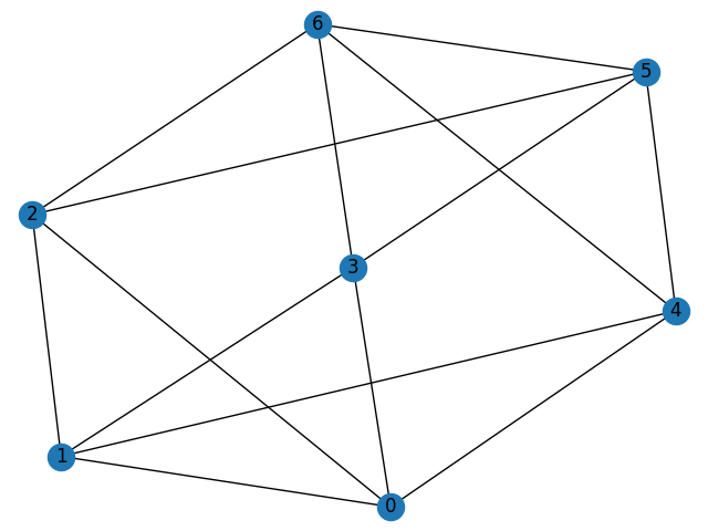
For this graph, optimal QAOA parameters read:

\[\gamma ^* \approx -0.240 \; ; \qquad \beta ^* \approx 0.327 \quad \Rightarrow \quad \left\langle H_\mathcal{C} \right\rangle ^* \approx -0.248\]

optimal_params = np.array([-0.240, 0.327])
optimal_cost = -0.248

We also define our cost operator \(H_{\mathcal{C}}\) as a function. Because it is diagonal in the computational basis, we only need to define its action on computational basis bitstrings.

def qaoa_cost(bitstring):

    bitstring = np.atleast_2d(bitstring)
    # Make sure that we operate correctly on a batch of bitstrings

    z = (-1) ** bitstring[:, graph.edges()]  # Filter out pairs of bits correspondimg to graph edges
    costs = z.prod(axis=-1).sum(axis=-1)  # Do products and sums
    return np.squeeze(costs) / len(graph.edges)  # Normalize

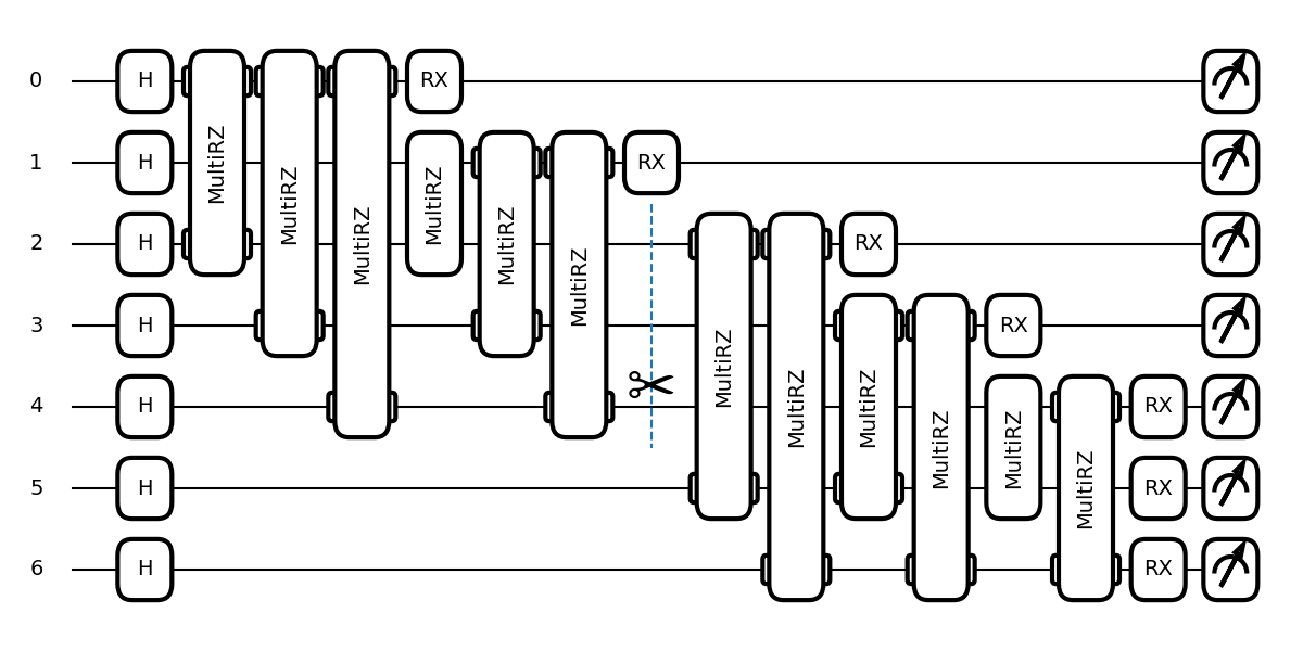
Let’s make a quick and simple QAOA circuit in PennyLane. Before we actually cut the circuit, we have to briefly think about the cut placement. First, we want to apply all ZZ rotation gates corresponding to the top_edges, place the wire cut, and then the bottom_edges, to ensure that the circuit actually splits in two after cutting.

def qaoa_template(params):

    gamma, beta = params

    for i in range(len(graph)):  # Apply the Hadamard gates
        qml.Hadamard(wires=i)

    for i, j in top_edges:

        # Apply the ZZ rotation gates
        # corresponding to the
        # green edges in the figure

        qml.MultiRZ(2 * gamma, wires=[i, j])

    qml.WireCut(wires=middle_nodes)  # Place the wire cut

    for i, j in bottom_edges:

        # Apply the ZZ rotation gates
        # corresponding to the
        # purple edges in the figure

        qml.MultiRZ(2 * gamma, wires=[i, j])

    for i in graph.nodes():  # Finally, apply the RX gates
        qml.RX(2 * beta, wires=i)

Let’s construct the QuantumTape corresponding to this template and draw the circuit:

from pennylane.tape import QuantumTape

all_wires = list(range(len(graph)))

with QuantumTape() as tape:
    qaoa_template(optimal_params)
    qml.sample(wires=all_wires)

fig, _ = qml.drawer.tape_mpl(tape, expansion_strategy="device")
fig.set_size_inches(12, 6)

The Pauli cutting method

To run fragment subcircuits and combine them into a finite-shot estimate of the optimal cost function using the Pauli cut method, we can use built-in PennyLane functions. We simply use the qml.cut_circuit_mc transform and everything is taken care of for us.

Note that we have already introduced the qml.cut_circuit transform in the previous section. The _mc appendix stands for Monte Carlo and is used to calculate finite-shot estimates of observables. The observable itself is passed to the qml.cut_circuit_mc transform as a function mapping a bitstring (circuit sample) to a single number.

dev = qml.device("default.qubit", wires=all_wires)


@qml.cut_circuit_mc(classical_processing_fn=qaoa_cost)
@qml.qnode(dev)
def qaoa(params):
    qaoa_template(params)
    return qml.sample(wires=all_wires)

We can obtain the cost estimate by simply running qaoa like a “normal” QNode. Let’s do just that for a grid of values so we can study convergence.

n_shots = 10000

shot_counts = np.logspace(1, 4, num=20, dtype=int, requires_grad=False)
pauli_cost_values = np.zeros_like(shot_counts, dtype=float)

for i, shots in enumerate(shot_counts):
    pauli_cost_values[i] = qaoa(optimal_params, shots=shots)

We will save these results for later and plot them together with results of the randomized measurement method.

The randomized channel-based cutting method

As noted earlier, the easiest way to mathematically represent the randomized channel-based method is to write down Kraus operators for the relevant channels, \(\Psi _0\) and \(\Psi _1\). Once we have represented them in explicit matrix form, we can simply use qml.QubitChannel.

To get our matrices, we represent the computational basis set along the \(k\) cut wires as a unit vector

\[\left\vert i \right\rangle \mapsto (0, \ldots, 1,\ldots,0)\]

with the 1 positioned at index \(i\). Therefore:

\[\begin{split}\left\vert i \right\rangle \left\langle j \right\vert \mapsto \begin{pmatrix} 0 & 0 & \cdots & 0 & 0 \\ 0 & \ddots & \cdots & 0 & 0 \\ \vdots & 0 & 1 & 0 & \vdots \\ 0 & 0 & \cdots & \ddots & 0 \\ 0 & 0 & \cdots & 0 & 0 \\ \end{pmatrix}\end{split}\]

where the 1 sits at column \(i\) and row \(j\).

Given this representation, a neat way to get all Kraus operators’ matrix representations is the following:

def make_kraus_ops(num_wires: int):

    d = 2**num_wires

    # High level idea: Take the identity operator on d^2 x d^2 and look at each row independently.
    # When reshaped into a matrix, it gives exactly the matrix representation of |i><j|:

    kraus0 = np.identity(d**2).reshape(d**2, d, d)

    kraus0 = np.concatenate([kraus0, np.identity(d)[None, :, :]], axis=0)
    # Add the identity op' to the mix

    kraus0 /= np.sqrt(d + 1)  # Normalize

    # Same trick for the other Kraus op'
    kraus1 = np.identity(d**2).reshape(d**2, d, d)
    kraus1 /= np.sqrt(d)

    # Finally, return a list of NumPy arrays, as per `qml.QubitChannel` docs.
    return list(kraus0.astype(complex)), list(kraus1.astype(complex))

Our next task is to generate two new QuantumTape objects from our existing tape, one for \(\Psi _0\) and one for \(\Psi _1\). Currently, a qml.WireCut dummy gate is used to represent the cut position and size. So, iterating through gates in tape:

• If the gate is a qml.WireCut, we apply the qml.QubitChannel corresponding to \(\Psi _0\) or \(\Psi _1\) to different new tapes.

• Otherwise, just apply the same existing gate to both new tapes.

In code, this looks like:

with QuantumTape(do_queue=False) as tape0, QuantumTape(do_queue=False) as tape1:
    # Record on new "fragment" tapes

    for op in tape:

        if isinstance(op, qml.WireCut):  # If the operation is a wire cut, replace it

            k = len(op.wires)
            d = 2**k

            K0, K1 = make_kraus_ops(k)  # Generate Kraus operators on the fly
            probs = (d + 1) / (2 * d + 1), d / (2 * d + 1)  # Probabilities of the two channels

            psi_0 = qml.QubitChannel(K0, wires=op.wires, do_queue=False)
            psi_1 = qml.QubitChannel(K1, wires=op.wires, do_queue=False)

            qml.apply(psi_0, context=tape0)
            qml.apply(psi_1, context=tape1)

        else:  # Otherwise, just apply the existing gate
            qml.apply(op, context=tape0)
            qml.apply(op, context=tape1)

Verify that we get expected values:

print(f"Cut size: k={k}")
print(f"Channel probabilities: p0={probs[0]:.2f}; p1={probs[1]:.2f}", "\n")

fig, _ = qml.drawer.tape_mpl(tape0, expansion_strategy="device")
fig.set_size_inches(12, 6)

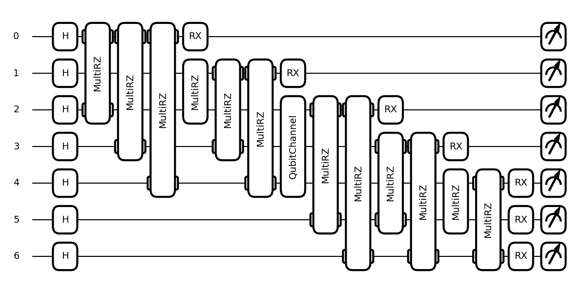
Out:

Cut size: k=3
Channel probabilities: p0=0.53; p1=0.47

You may have noticed that both generarated tapes have the same size as the original tape. It may seem that no circuit cutting actually took place. However, this is just an artifact of the way we chose to represent classical communication between subcircuits. Measure-and-prepare channels at work here are more naturally implemented on a mixed-state simulator. On a real quantum device however, introducing a classical communication step is equivalent to separating the circuit into two.

Given that we are dealing with quantum channels, we need a mixed-state simulator. Luckily, PennyLane has just what we need:

device = qml.device("default.mixed", wires=tape.wires)

We only need a single run each of the two generated tapes, tape0 and tape1, collecting the appropriate number of samples. NumPy can take care of this for us - we let np.choice make our decision on which tape to run for each shot:

samples = np.zeros((n_shots, len(tape.wires)), dtype=int)

rng = np.random.default_rng(seed=1337)
choices = rng.choice(2, size=n_shots, p=probs)

channels, channel_shots = np.unique(choices, return_counts=True)

print("Which channel to run:", choices)
print(f"Channel 0: {channel_shots[0]} times")
print(f"Channel 1: {channel_shots[1]} times.")

Out:

Which channel to run: [1 0 1 ... 0 1 0]
Channel 0: 5305 times
Channel 1: 4695 times.

Time to run the simulator!

device.shots = channel_shots[0].item()
(shots0,) = qml.execute([tape0], device=device, cache=False, gradient_fn=None)
samples[choices == 0] = shots0

device.shots = channel_shots[1].item()
(shots1,) = qml.execute([tape1], device=device, cache=False, gradient_fn=None)
samples[choices == 1] = shots1

Now that we have the result stored in samples, we still need to do some post-processing to obtain final estimates of the QAOA cost. In the case of a single cut, the resolution of the identity discussed earlier implies

\[\left\langle H_\mathcal{C} (x) \right\rangle = (d +1) \left\langle H_\mathcal{C} (x) \right\rangle _{z=0} - d \left\langle H_\mathcal{C} (x) \right\rangle _{z=1},\]

where \(d=2^k\) and \(z=0,1\) corresponds to circuits with inserted channels \(\Psi _{0,1}\).

d = 2**k

randomized_cost_values = np.zeros_like(pauli_cost_values)

signs = np.array([1, -1], requires_grad=False)
shot_signs = signs[choices]

for i, cutoff in enumerate(shot_counts):
    costs = qaoa_cost(samples[:cutoff])
    randomized_cost_values[i] = (2 * d + 1) * np.mean(shot_signs[:cutoff] * costs)

Let’s plot the results comparing the two methods:

import matplotlib.pyplot as plt

fig, ax = plt.subplots(figsize=(12, 6))

ax.semilogx(
    shot_counts,
    pauli_cost_values,
    "o-",
    c="darkorange",
    ms=8,
    markeredgecolor="k",
    label="Pauli",
)

ax.semilogx(
    shot_counts,
    randomized_cost_values,
    "o-",
    c="steelblue",
    ms=8,
    markeredgecolor="k",
    label="Randomized",
)

ax.axhline(optimal_cost, color="k", linestyle="--", label="Exact value")

ax.tick_params(axis="x", labelsize=18)
ax.tick_params(axis="y", labelsize=18)

ax.set_ylabel("QAOA cost", fontsize=20)
ax.set_xlabel("Number of shots", fontsize=20)

_ = ax.legend(frameon=True, loc="lower right", fontsize=20)

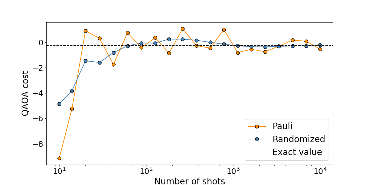
We see that the randomized method converges faster than the Pauli method - fewer shots will get us a better estimate of the true cost function. This is even more apparent when we increase the number of shots and go to larger graphs and/or QAOA depths \(p\). For example, here are some results that include cost variances as well as mean values for a varying number of shots.

Figure 6. An example of QAOA cost convergence for a circuit cut both with the Pauli method and randomized channel method.

The randomized method offers a quadratic overhead reduction. In practice, for larger cuts, we see that it offers a performance that is orders of magnitude better than that of the Pauli method. For larger circuits, even at \(10^6\) shots, Pauli estimates still sometimes leave the allowed interval of \([-1,1]\).

However, these improvements come at the cost of increased circuit depth due to inserting random Clifford gates and additional classical communication required.

Multiple cuts and mid-circuit measurements

Careful readers may have noticed that QAOA at depth \(p=1\) has a specific structure of a Matrix Product State (MPS) circuit. However, in order to cut a \(p=2\) QAOA circuit, we would need 2 cuts. This introduces some subtleties within the context of classical simulation that we point out here.

The measurement performed as a part of the first cut always induces a reduced state on the remaining wires. If the circuit has an MPS structure, we can just measure all qubits at once —a part of the measured bitstring gets passed into the second fragment and the remaining bits go directly into the output bitstring. However, when we try the same thing on a non-MPS circuit, additional gates need to be applied on the wires that now hold a reduced state. This is the other reason why it is easier to simulate circuit cutting of a non-MPS circuit with a mixed-state simulator.

Figure 7. A schematic representation of the mid-circuit measurement “problem”.

Note that, in these cases, memory requirements of classical simulation are increased from \(O(2^n)\) to \(O(4^n)\). However, this is only a constraint for classical simulation where we have to choose between state-vector and density-matrix approaches. Real quantum devices don’t have such limitations, of course.

References

1

T. Peng, A. Harrow, M. Ozols, and X. Wu (2019) “Simulating Large Quantum Circuits on a Small Quantum Computer”. (arXiv)

2(1,2)

A. Lowe et. al. (2022) “Fast quantum circuit cutting with randomized measurements”. (arXiv)

About the authors

Gideon Uchehara

Gideon is a PhD student at the University of British Columbia, Canada. His research is in quantum algorithms and quantum machine learning. He works at Xanadu as a Quantum Computing Educator Intern. He recently started the Blacks In Quantum (BIQ) initiative and also serves as the student representative on the International Program Committee for the Quantum Computing NSERC CREATE Program, British Columbia, Canada.

Matija Medvidović

Matija is a PhD student at Columbia University and the Flatiron Institute in New York. He works with machine learning methods to study quantum many-body physics and quantum computers. He is currently a part of the Xanadu Residency Program. He is a firm believer in keeping bios short and concise.

Anuj Apte

Anuj is a PhD student at the University of Chicago. His research interests include quantum field theory with applications to topological phases and quantum computing.

demos/tutorial_quantum_circuit_cutting

 

Download Python script

 

Download Notebook

 

View on GitHub