Testing for symmetry with quantum computers

Author: David Wakeham. Posted: 24 January 2023.

Symmetries are transformations that leave something looking the same. They are not only pretty — think of geometric patterns and shapes — but a great labour-saving device for the lazy physicist! You can do something once, and by applying transformations, find your work has been multiplied ten-fold. Symmetries need not be exact, since a system can look approximately, rather than exactly, the same after a transformation. It therefore makes sense to have an algorithm to determine if a Hamiltonian, encoding the physics of a quantum system, has an approximate symmetry.

In this demo, we’ll implement the elegant algorithm of LaBorde and Wilde (2022) for testing the symmetries of a Hamiltonian. We’ll be able to determine whether a system has a finite group of symmetries \(G\), and if not, by how much the symmetry is violated.

Background

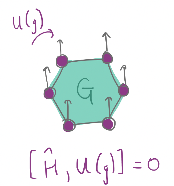
We will encode symmetries into a finite group. This is an algebraic structure consisting of transformations \(g\), which act on the Hilbert space \(\mathcal{H}\) of our system in the form of unitary operators \(U(g)\) for \(g \in G\). More formally, given any two elements \(g_1, g_2\in G\), there is a product \(g_1 \circ g_2 \in G\), and such that:

• multiplication is associative, \(g_1 \circ (g_2 \circ g_3) = (g_1 \circ g_2) \circ g_3\) for all \(g_1, g_2, g_3 \in G\);

• there is a boring transformation \(e\) that does nothing, \(g \circ e = e \circ g = e\) for all \(g \in G\);

• transformations can be undone, with some \(g^{-1} \in G\) such that \(g \circ g^{-1} = g^{-1} \circ g = e\) for all \(g \in G\).

It is sensible to ask that the unitary operators preserve the structure of the group:

\[U(g_1)U(g_2) = U(g_1 \circ g_2).\]

For more on groups and how to represent them with matrices, see our demo on geometric learning. For the Hamiltonian to respect the symmetries encoded in the group \(G\) it means that it commutes with the matrices,

\[[U(g),\hat{H}] = 0\]

for all \(g \in G\). Since the Hamiltonian generates time evolution, this means that if we apply a group transformation now or we apply it later, the effect is the same. Thus, we seek an algorithm which checks if these commutators are zero.

Averaging over symmetries

To verify that the Hamiltonian is symmetric with respect to \(G\), it seems like we will need to check each element \(g \in G\) separately. There is a clever way to avoid this and boil it all down to a single number. For now, we’ll content ourselves with looking at the average over the group:

\[\frac{1}{|G|}\sum_{g\in G}[U(g),\hat{H}] = 0.\]

To make things concrete, let’s consider the cyclic group \(G = \mathbb{Z}_4\), which we can think of as rotations of the square. If we place a qubit on each corner, this group will naturally act on four qubits.

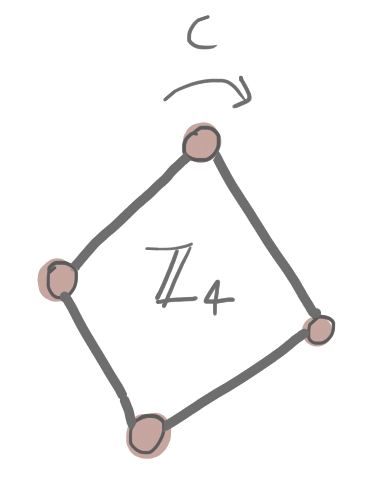
It is generated by a single rotation, which we’ll call \(c\). We’ll consider three Hamiltonians: one which is exactly symmetric with respect to \(G\) (called \(\hat{H}_\text{symm}\)), one which is near symmetric (called \(\hat{H}_\text{nsym}\)), and one which is asymmetric (called \(\hat{H}_\text{asym}\)). We’ll define them by

\[\begin{split}\begin{align*} \hat{H}_\text{symm} & = X_0 + X_1 + X_2 + X_3\\ \hat{H}_\text{nsym} & = X_0 + 1.1 \cdot X_1 + 0.9 \cdot X_2 + X_3 \\ \hat{H}_\text{asym} & = X_0 + 2\cdot X_1 + 3\cdot X_2. \end{align*}\end{split}\]

Let’s see how this looks in PennyLane. We’ll create a register system with four wires, one for each qubit. The generator \(c\) acts as a permutation:

\[\vert x_0 x_1 x_2 x_3\rangle \overset{c}{\mapsto} \vert x_3 x_0 x_1 x_2\rangle\]

for basis states \(\vert x_0 x_1 x_2 x_3\rangle\) and extends by linearity. The simplest way to do this is by using qml.Permute. We can convert this into a matrix by using qml.matrix(). We can obtain any other element \(g\in G\) by simply iterating \(c\) the appropriate number of times.

import pennylane as qml
from pennylane import numpy as np

# Create wires for the system
system = range(4)

# The generator of the group
c = qml.Permute([3, 0, 1, 2], wires=system)
c_mat = qml.matrix(c)

To create the Hamiltonians, we use qml.Hamiltonian:

# Create Hamiltonians
obs = [qml.PauliX(system[0]), qml.PauliX(system[1]), qml.PauliX(system[2]), qml.PauliX(system[3])]
coeffs1, coeffs2, coeffs3 = [1, 1, 1, 1], [1, 1.1, 0.9, 1], [1, 2, 3, 0]
Hsymm, Hnsym, Hasym = (
    qml.Hamiltonian(coeffs1, obs),
    qml.Hamiltonian(coeffs2, obs),
    qml.Hamiltonian(coeffs3, obs),
)

To arrive at the algorithm for testing this average symmetry property, we start with a trick called the Choi-Jamiołkowski isomorphism for thinking of time evolution as a state instead of an operator. This state is called the dual of the operator. It’s easy to describe how to construct this state in words: make a copy \(\mathcal{H}_\text{copy}\) of the system \(\mathcal{H}\), create a maximally entangled state, and time evolve the state on \(\mathcal{H}\). In fact, this trick works to give a dual state \(\vert\Phi^U\rangle\) for any operator \(U\), as below:

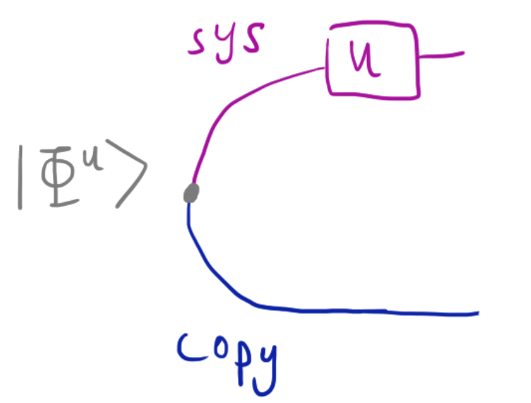
We’ve pictured entanglement by joining the wires corresponding to the system and the copy. For time evolution, we’ll call the dual state \(\vert\Phi_t\rangle\), and formally define it:

\[\vert\Phi_t\rangle = \frac{1}{\sqrt{d}}\sum_{i=1}^d e^{-it\hat{H}}\vert i\rangle \otimes \vert i_\text{copy}\rangle.\]

You can show mathematically that the average symmetry condition is equivalent to

\[\Pi_G\vert\Phi_t\rangle = \vert\Phi_t\rangle,\]

where \(\Pi_G\) is an operator defined by

\[\Pi_G = \frac{1}{|G|}\sum_{g\in G} U(g) \otimes \overline{U(g)}.\]

In fact, it turns out that \(\Pi_G^2 = \Pi_G\), and hence it is a projector, with an associated measurement, asking: is the state symmetric on average? The statement \(\Pi_G \vert \Psi_t\rangle = \vert \Psi_t \rangle\) is a mathematical way of saying “yes”. So, our goal now is to write a circuit which (a) prepares the state \(\vert\Phi_t\rangle\), and (b) performs the measurement \(\Pi_G\). Part (a) is simpler — in general, we can just use a “cascade” of Hadamards and CNOTs, similar to the usual circuit for generating a Bell state on two qubits, as pictured below:

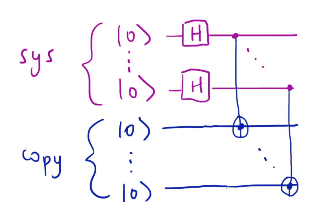
Let’s implement this for our four-qubit system in PennyLane:

# Create copy of the system
copy = range(4, 8)

# Prepare entangled state on system and copy
def prep_entangle():
    for wire in system:
        qml.Hadamard(wire)
        qml.CNOT(wires=[wire, wire + 4])

We then need to implement time evolution on the system. In applications, the system’s evolution could be a “black box” we can query, or something given to us analytically. In general, we can approximate time evolution with qml.ApproxTimeEvolution. However, since our Hamiltonians consist of terms that commute, we will be able to evolve exactly using qml.CommutingEvolution. We will reiterate this below. That’s it for part (a)!

# Use Choi-Jamiołkowski isomorphism
def choi_state(hamiltonian, time):
    prep_entangle()
    qml.CommutingEvolution(hamiltonian, time)

Controlled symmetries

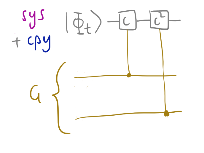
Part (b) is more interesting. The simplest approach is to use an auxiliary register \(\mathcal{H}_G\) which encodes \(G\), with basis elements \(\vert g\rangle\) labelled by group elements \(g \in G\). This needs \(\log \vert G\vert\) qubits, which (along with any Hamiltonian simulation) will form the main resource cost of the algorithm. These will then can group transformations to a state \(\vert\psi\rangle \in \mathcal{H}\otimes \mathcal{H}_\text{copy}\) in a controlled way via

\[\vert{\psi}\rangle \otimes \vert g\rangle \mapsto (U(g)\otimes \overline{U(g)})\vert{\psi} \rangle \otimes \vert g\rangle_G,\]

which we’ll call \(CU\). We take this controlled gate as a primitive. To test average symmetry, we simply place \(\mathcal{H}_G\) in a uniform superposition

\[\vert +\rangle_G = \frac{1}{\sqrt{|G|}}\sum_{g\in G} \vert g\rangle_G\]

and apply the controlled operator to the state generated in part (a). This gives

\[\vert\Phi_t\rangle \otimes \vert +\rangle_G \mapsto \frac{1}{\sqrt{|G|}}\sum_{g\in G}(U(g)\otimes \overline{U(g)})\vert\Phi_t\rangle \otimes \vert g\rangle_G.\]

This isn’t quite what we want yet, in particular because the system \(\mathcal{H}\) is entangled not only with the copy, but also with the register \(\mathcal{H}_G\). To fix this, we observe the register, and see if it’s in the superposition \(\vert+\rangle_G\). The state, conditioned on this observation, is

\[\begin{split}\begin{align*} {}_G\langle +\vert \frac{1}{\sqrt{|G|}}\sum_{g\in G}(U(g)\otimes \overline{U(g)})\vert\Phi_t\rangle \otimes \vert g\rangle_G & = \frac{1}{|G|}\sum_{g, g'\in G}(U(g)\otimes \overline{U(g)})\vert\Phi_t\rangle \langle g'\vert g\rangle_G \\ & = \Pi_G \vert\Phi_t\rangle, \end{align*}\end{split}\]

and hence the probability of observing it is

\[P_+ = \vert \Pi_G \vert\Phi_t\rangle \vert^2 = \langle \Phi_t \vert \Pi_G^\dagger \Pi_G\vert\Phi_t\rangle = \langle \Phi_t \vert \Pi_G\vert\Phi_t\rangle\]

This is exactly what we want! So, let’s code all this up for our example. We’ll need two qubits for our auxiliary register \(\mathcal{H}_G\). To place it in a uniform superposition, just apply a Hadamard gate to each qubit. To measure the \(\vert+\rangle_G\) state at the end, we undo these Hadamards and try to measure “\(00\)”. Finally, it’s straightforward to implement the controlled gate \(CU\) using controlled operations (namely qml.ControlledQubitUnitary) on each qubit:

# Create group register and device
aux = range(8, 10)
dev = qml.device("default.qubit", wires=10)

# Create plus state
def prep_plus():
    qml.Hadamard(wires=aux[0])
    qml.Hadamard(wires=aux[1])

# Implement controlled symmetry operations on system
def CU_sys():
    qml.ControlledQubitUnitary(c_mat @ c_mat, control_wires=[aux[0]], wires=system)
    qml.ControlledQubitUnitary(c_mat, control_wires=[aux[1]], wires=system)


# Implement controlled symmetry operations on copy
def CU_cpy():
    qml.ControlledQubitUnitary(c_mat @ c_mat, control_wires=[aux[0]], wires=copy)
    qml.ControlledQubitUnitary(c_mat, control_wires=[aux[1]], wires=copy)

Let’s combine everything and actually run our circuit!

# Circuit for average symmetry
@qml.qnode(dev, interface="autograd")
def avg_symm(hamiltonian, time):

    # Use Choi-Jamiołkowski isomorphism
    choi_state(hamiltonian, time)

    # Apply controlled symmetry operations
    prep_plus()
    CU_sys()
    CU_cpy()

    # Ready register for measurement
    prep_plus()

    return qml.probs(wires=aux)


print("For Hamiltonian Hsymm, the |+> state is observed with probability", avg_symm(Hsymm, 1)[0], ".")
print("For Hamiltonian Hnsym, the |+> state is observed with probability", avg_symm(Hnsym, 1)[0], ".")
print("For Hamiltonian Hasym, the |+> state is observed with probability", avg_symm(Hasym, 1)[0], ".")

Out:

For Hamiltonian Hsymm, the |+> state is observed with probability 1.0000000000000007 .
For Hamiltonian Hnsym, the |+> state is observed with probability 0.9802155808358518 .
For Hamiltonian Hasym, the |+> state is observed with probability 0.2249891886216874 .

We see that for the symmetric Hamiltonian, we’re certain to observe \(\vert +\rangle_G\). We’re very likely to observe \(\vert +\rangle_G\) for the near-symmetric Hamiltonian, and our chances suck for the asymmetric Hamiltonian.

A short time limit

This circuit leaves a few things to be desired. First, it only measures whether our Hamiltonian is symmetric on average. What if we want to know if it’s symmetric with respect to each element individually? We could run the circuit for each element \(g\in G\), but perhaps there is a better way. Second, even if we could do that, we don’t know what the numbers coming out of the circuit mean. We can address both questions by considering very short times, \(t \to 0\). In this case, we can Taylor expand the unitary time-evolution operator,

\[e^{-it \hat{H}} = \mathbb{I} - it \hat{H} - \frac{t^2 \hat{H}^2}{2} + O(t^3).\]

We’ll assume that, if we’re simulating the evolution, the expansion is accurate to this order. Also, let \(d\) be the dimension of our system. In this case, it’s possible to prove that the probability \(P_+\) of observing the \(\vert +\rangle_G\) state is

\[P_+ = \langle \Phi_t \vert \Pi_G \vert \Phi_t\rangle = 1 - \frac{t^2}{2d \vert G\vert}\sum_{g\in G}\vert\vert [U(g), \hat{H}] \vert\vert_2^2 + O(t^3),\]

where \(\vert\vert\cdot\vert\vert_2\) represents the usual (Pythagorean) \(2\)-norm. This is a sharp expression relating the output of the circuit \(P_+\) to a quantity measuring the degree of symmetry or lack thereof, the sum of squared commutator norms. We’ll call this sum the asymmetry \(\xi\). Rearranging, we have

\[\xi = \sum_{g\in G}\vert\vert [U(g), \hat{H}] \vert\vert_2^2 = \frac{2d\vert G\vert(1 - P_+)}{t^2} + O(t).\]

Let’s see how this works in our example. Since \(d\) is the dimension of the system, in our four-qubit case, \(d=2^4 = 16\), while \(\vert G\vert = 4\).

# Define asymmetry circuit
def asymm(hamiltonian, time):
    d, G = 16, 4
    P_plus = avg_symm(hamiltonian, time)[0]
    xi = 2 * d * (1 - P_plus) / (time ** 2)
    return xi


print("The asymmetry for Hsymm is", asymm(Hsymm, 1e-4), ".")
print("The asymmetry for Hnsym is", asymm(Hnsym, 1e-4), ".")
print("The asymmetry for Hasym is", asymm(Hasym, 1e-4), ".")

Out:

The asymmetry for Hsymm is 1.2079226507921703e-05 .
The asymmetry for Hnsym is 0.6400121321803454 .
The asymmetry for Hasym is 159.99999902760464 .

Our symmetric Hamiltonian \(\hat{H}_\text{symm}\) has a near-zero asymmetry as expected. The near-symmetric Hamiltonian \(\hat{H}_\text{nsym}\) has an asymmetry much larger than \(O(t)\); evidently, \(\xi\) is a more intelligible measure of symmetry than \(P_+\). Finally, the Hamiltonian \(\hat{H}_\text{asym}\) has a huge error; it is not even approximately symmetric.

Concluding remarks

Symmetries are physically important in quantum mechanics. Most systems of interest are large and complex, and even with an explicit description of a Hamiltonian, symmetries can be hard to determine by hand. Testing for symmetry when we have access to Hamiltonian evolution (either physically or by simulation) is thus a natural target for quantum computing.

Here, we’ve described a simple algorithm to check if a system with Hamiltonian \(\hat{H}\) is approximately symmetric with respect to a finite group \(G\). More precisely, for short times, applying controlled symmetry operations to the state dual to Hamiltonian evolution gives the asymmetry

\[\xi = \sum_{g\in G} \vert\vert [U(g), H]\vert\vert^2_2.\]

This vanishes just in case the system possesses the symmetry, and otherwise tells us by how much it is violated. The main overhead is the size of the register encoding the group, which scales logarithmically with \(\vert G\vert\). So, it’s expensive in memory for big groups, but quick to run! Regardless of the details, this algorithm suggests routes for further exploring the rich landscape of symmetry with quantum computers.

References

1. LaBorde, M. L and Wilde, M.M. Quantum Algorithms for Testing Hamiltonian Symmetry (2022).

About the author

David Wakeham

David's elements formed from exploding stars billions of years ago but self-organized into a human more recently. He has a background in string theory and particle physics, but decided his life would be better spent making colourful widgets. His personal website is hapax.github.io.

demos/tutorial_testing_symmetry

 

Download Python script

 

Download Notebook

 

View on GitHub