Modeling the toric code on a quantum computer

Author: Christina Lee. Posted: 08 August 2022.

Introduction

The toric code model 1 is a treasure trove of interesting physics and mathematics. The model sparked the development of the error-correcting surface codes 2, an essential category of error correction models. But why is the model so useful for error correction?

We delve into mathematics and condensed matter physics to answer that very question. Viewing the model as a description of spins in an exotic magnet allows us to start analyzing the model as a material. What kind of material is it? The toric code is an example of a topological state of matter.

A state of matter, or phase, cannot become a different phase without some discontinuity in the physical properties as coefficients in the Hamiltonian change. This discontinuity may exist in an arbitrary order derivative or non-local observable. For example, ice cannot become water without a discontinuity in density as the temperature changes. The ground state of a topological state of matter cannot smoothly deform to a non-entangled state without a phase transition. Entanglement, and more critically long-range entanglement, is a key hallmark of a topological state of matter.

Local measurements cannot detect topological states of matter. We have to consider the entire system to determine a topological phase. To better consider this type of property, consider the parity of the number of dancers on a dance floor. Does everyone have a partner, or is there an odd person out? To measure that, we have to look at the entire system.

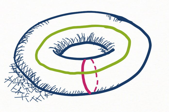
Topology is the study of global properties that are preserved under continuous deformations. For example, a coffee cup is equivalent to a donut because they both have a single hole. More technically, they both have an Euler characteristic of zero. When we zoom to a local patch, both a sphere and a torus look the same. Only by considering the object as a whole can you detect the single hole.

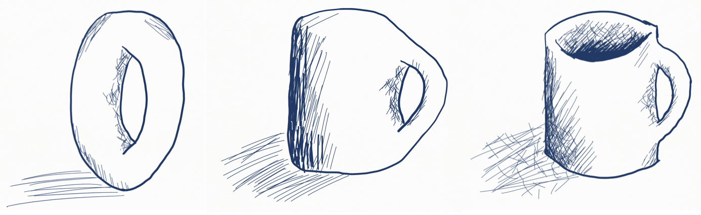
A donut can be smoothly deformed into a mug.

In this demo, we will look at the degenerate ground state and the excitations of the toric code model. The toric code was initially proposed in “Fault-tolerant quantum computation by anyons” by Kitaev 1. This demo was inspired by “Realizing topologically ordered states on a quantum processor” by K. J. Satzinger et al 3. For further reading, I recommend “Quantum Spin Liquids” by Lucile Savary and Leon Balents 4 and “A Pedagogical Overview on 2D and 3D Toric Codes and the Origin of their Topological Orders” 5.

The Model

What is the source of all this fascinating physics? The Hamiltonian is:

\[\mathcal{H} = -\sum_s S_s - \sum_p P_p,\]

where

\[S_s = \prod_{i \in s} Z_i \quad P_p = \prod_{j \in p} X_j.\]

In the literature, the \(S_s\) terms are called the “star” operators, and the \(P_p\) terms are called the “plaquette” operators. Each star \(s\) and plaquette \(p\) is a group of 4 sites on a square lattice. You can compare this model to something like the Heisenberg model used to describe spins interacting magnetically in a material.

In the most common formulation of the model, sites live on the edges of a square lattice. In this formulation, the “plaquette” operators are products of Pauli X operators on all the sites in a square, and the “star” operators are products of Pauli Z operators on all the sites bordering a vertex.

Instead, we can view the model as a checkerboard of alternating square types. In this formulation, all sites \(i\) and \(j\) are the vertices of a square lattice. Each square is a group of four sites, and adjacent squares alternate between the two types of groups. Since the groups on this checkerboard no longer look like stars and plaquettes, we will call them the “Z Group” and “X Group” operators in this tutorial.

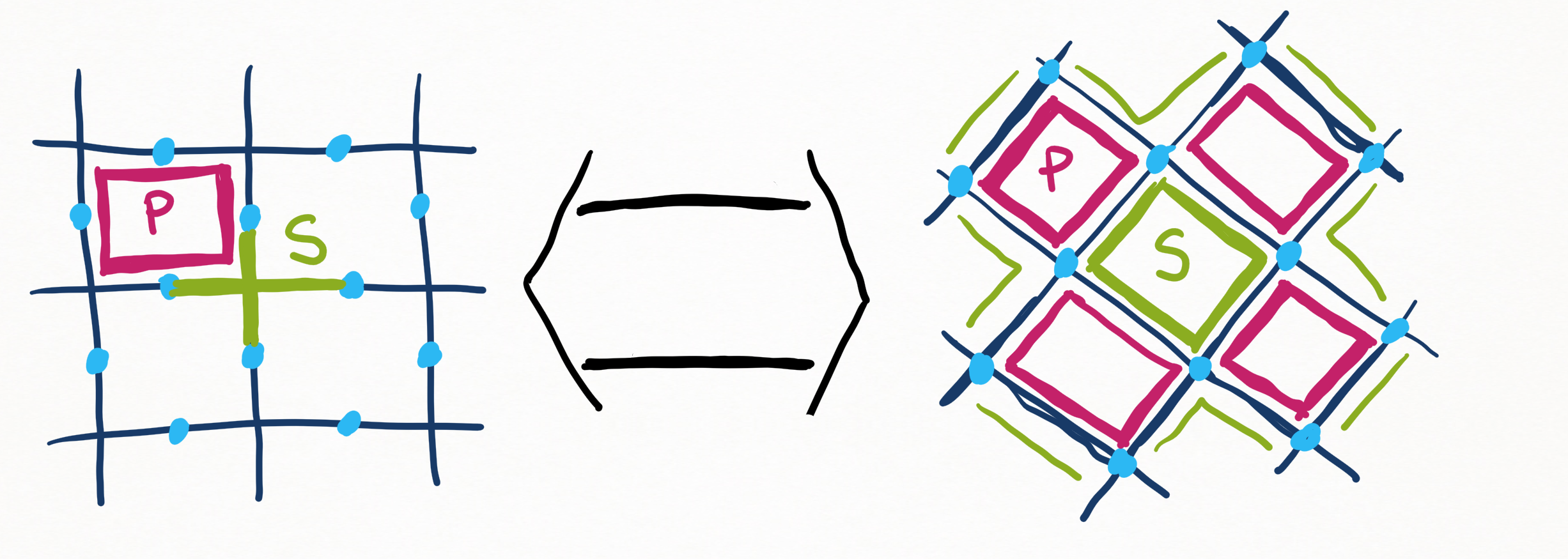
On the left, sites are grouped into stars around vertices and plaquettes on the faces. On the right, we view the lattice as a checkerboard of alternating types of groups.

We will be embedding the lattice on a torus via periodic boundary conditions. Periodic boundary conditions basically “glue” the bottom of the lattice to the top of the lattice and the left to the right.

Modular arithmetic accomplishes this matching. Any site at (x,y) is the same as a site at (x+width, y+height).

By matching up the edges with periodic boundary conditions, we turn a square grid into a torus.

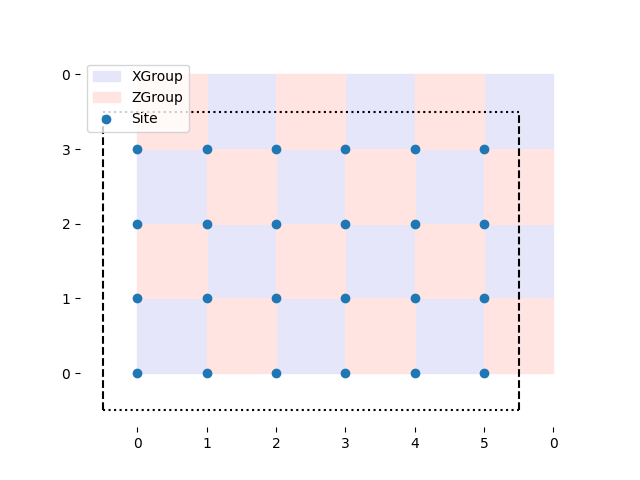
On to some practical coding! First, let’s define the sites on a \(4\times 6\) lattice.

import pennylane as qml
import matplotlib.pyplot as plt
from matplotlib.patches import Polygon, Patch
from itertools import product
from dataclasses import dataclass

import numpy as np

np.set_printoptions(suppress=True)

height = 4
width = 6

all_sites = [(i, j) for i, j in product(range(width), range(height))]

We would like for our wire labels to match the sites. To do this, we will be using an Immutable Data Class . PennyLane allows wire labels to be any hashable object, but iterable wire labels are currently not supported. Therefore we use a frozen dataclass to represent individual wires by a row and column position.

@dataclass(frozen=True)
class Wire:
    i: int
    j: int

example_wire = Wire(0, 0)
print("Example wire: ", example_wire)
print("At coordinates: ", example_wire.i, example_wire.j)

Out:

Example wire:  Wire(i=0, j=0)
At coordinates:  0 0

Setting up Operators

For each type of group operator (X and Z), we will have two different lists: the “sites” and the “ops”. The “sites” are tuples and will include virtual sites off the edge of the lattice that match up with locations on the other side. For example, the site (6, 1) denotes the real location (0,1). We will use the zgroup_sites and xgroup_sites lists to help us view the measurements of the corresponding operators.

The “ops” list will contain the tensor observables. We will later take the expectation value of each tensor.

mod = lambda s: Wire(s[0] % width, s[1] % height)

zgroup_sites = []  # list of sites in each group
zgroup_ops = []  # list of operators for each group

for x, y in product(range(width // 2), range(height)):

    x0 = 2 * x + (y + 1) % 2 # x starting coordinate

    sites = [(x0, y), (x0 + 1, y), (x0 + 1, y + 1), (x0, y + 1)]

    op = qml.operation.Tensor(*(qml.PauliZ(mod(s)) for s in sites))

    zgroup_sites.append(sites)
    zgroup_ops.append(op)

print("First set of sites: ", zgroup_sites[0])
print("First operator: ", zgroup_ops[0])

Out:

First set of sites:  [(1, 0), (2, 0), (2, 1), (1, 1)]
First operator:  PauliZ(wires=[Wire(i=1, j=0)]) @ PauliZ(wires=[Wire(i=2, j=0)]) @ PauliZ(wires=[Wire(i=2, j=1)]) @ PauliZ(wires=[Wire(i=1, j=1)])

We will later use the X Group operator sites to prepare the ground state, so the order here is important. One group needs a slightly different order due to interference with the periodic boundary condition.

xgroup_sites = []
xgroup_ops = []
for x, y in product(range(width // 2), range(height)):
    x0 = 2 * x + y % 2 # lower x coordinate

    sites = [(x0 + 1, y + 1), (x0, y + 1), (x0, y), (x0 + 1, y)]

    if x == 2 and y == 1:  # change order for state prep later
        sites = sites[1:] + sites[0:1]

    op = qml.operation.Tensor(*(qml.PauliX(mod(s)) for s in sites))

    xgroup_sites.append(sites)
    xgroup_ops.append(op)

How can we best visualize these groups of four sites?

We use matplotlib to show each group of four sites as a Polygon patch, coloured according to the type of group. The misc_plot_formatting function performs some minor styling improvements repeated throughout this demo. The dotted horizontal lines and dashed vertical lines denote where we glue our boundaries together.

def misc_plot_formatting(fig, ax):
    plt.hlines([-0.5, height - 0.5], -0.5, width - 0.5, linestyle="dotted", color="black")
    plt.vlines([-0.5, width - 0.5], -0.5, height - 0.5, linestyle="dashed", color="black")
    plt.xticks(range(width + 1), [str(i % width) for i in range(width + 1)])
    plt.yticks(range(height + 1), [str(i % height) for i in range(height + 1)])

    for direction in ["top", "right", "bottom", "left"]:
        ax.spines[direction].set_visible(False)

    return fig, ax


fig, ax = plt.subplots()
fig, ax = misc_plot_formatting(fig, ax)

for group in xgroup_sites:
    x_patch = ax.add_patch(Polygon(group, color="lavender", zorder=0))

for group in zgroup_sites:
    z_patch = ax.add_patch(Polygon(group, color="mistyrose", zorder=0))

plt_sites = ax.scatter(*zip(*all_sites))

plt.legend([x_patch, z_patch, plt_sites], ["XGroup", "ZGroup", "Site"], loc="upper left")

plt.show()

The Ground State

While individual X and Z operators do not commute with each other, the X Group and Z Group operators do:

\[[S_s, P_p] = 0.\]

Since they commute, the wavefunction can be an eigenstate of each group operator independently. To minimize the energy of the Hamiltonian on the system as a whole, we can minimize the contribution of each group operator. Due to the negative coefficients in the Hamiltonian, we need to maximize the expectation value of each operator. The maximum possible expectation value for each operator is \(+1\). We can turn this into a constraint on our ground state:

\[S_s |G \rangle = +1 |G \rangle \qquad \qquad P_p | G \rangle = +1 |G\rangle.\]

The wavefunction

\[| G \rangle = \prod_{p} \frac{\mathbb{I} + P_p}{\sqrt{2}} |00\dots 0\rangle = \prod_{p} U_p |00\dots 0 \rangle,\]

where \(P_p\) (plaquette) denotes an X Group operator, is such a state.

Note

To check your understanding, confirm that this ground state obeys the constraints using pen and paper.

\(|G \rangle\) contains a product of unitaries \(U_p\). If we can figure out how to apply a single \(U_p\) using a quantum computer’s operations, we can apply that decomposition for every \(p\) in the product.

To better understand how to decompose \(U_p\), let’s write it concretely for a single group of four qubits:

\[U |0000 \rangle = \frac{\left(\mathbb{I} + X_1 X_2 X_3 X_4 \right)}{\sqrt{2}} |0000 \rangle = \frac{1}{\sqrt{2}} \left( |0000\rangle + |1111\rangle \right).\]

This generalized GHZ state can be prepared with a Hadamard and 3 CNOT gates:

This decomposition for \(U_p\) holds only when the initial Hadamard qubit begins in the \(|0\rangle\) state, so we need to be careful in the choice of the Hadamard’s qubit. This restriction is why we rotated the order for a single X Group on the right border earlier.

We will also not need to prepare the final X Group that contains the four edges of the lattice.

Now let’s actually put these together into a circuit!

dev = qml.device("lightning.qubit", wires=[Wire(*s) for s in all_sites])

def state_prep():
    for op in xgroup_ops[0:-1]:
        qml.Hadamard(op.wires[0])
        for w in op.wires[1:]:
            qml.CNOT(wires=[op.wires[0], w])

@qml.qnode(dev, diff_method=None)
def circuit():
    state_prep()
    return [qml.expval(op) for op in xgroup_ops + zgroup_ops]

From this QNode, we can calculate the group operators’ expectation values and the system’s total energy.

n_xgroups = len(xgroup_ops)
separate_expvals = lambda expvals: (expvals[:n_xgroups], expvals[n_xgroups:])

xgroup_expvals, zgroup_expvals = separate_expvals(circuit())

E0 = -sum(xgroup_expvals) - sum(zgroup_expvals)

print("X Group expectation values", [np.round(val) for val in xgroup_expvals])
print("Z Group expectation values", [np.round(val) for val in zgroup_expvals])
print("Total energy: ", E0)

Out:

X Group expectation values [1.0, 1.0, 1.0, 1.0, 1.0, 1.0, 1.0, 1.0, 1.0, 1.0, 1.0, 1.0]
Z Group expectation values [1.0, 1.0, 1.0, 1.0, 1.0, 1.0, 1.0, 1.0, 1.0, 1.0, 1.0, 1.0]
Total energy:  -23.999999999999996

Excitations

Quasiparticles allow physicists to describe complex systems as interacting particles in a vacuum. Examples of quasiparticles include electrons and holes in semiconductors, phonons, and magnons.

Imagine trying to describe the traffic on the road. We could either explicitly enumerate the location of each vehicle or list the positions and severities of traffic jams.

The first option provides complete information about the system but is much more challenging to analyze. For most purposes, we can work with information about how the traffic deviates from a baseline. In semiconductors, we don’t write out the wave function for every single electron. We instead use electrons and holes. Neither quasiparticle electrons nor holes are fundamental particles like an electron or positron in a vacuum. Instead, they are useful descriptions of how the wave function differs from its ground state.

While the electrons and holes of a metal behave just like electrons and positrons in a vacuum, some condensed matter systems contain quasiparticles that cannot or do not exist as fundamental particles. The excitations of the toric code are one such example. To find these quasiparticles, we look at states that are almost the ground state, such as the ground state with a single operator applied to it.

Suppose we apply a perturbation to the ground state in the form of a single X gate at location \(i\) :

\[| \phi \rangle = X_i | G \rangle.\]

Two Z group operators \(S_s\) contain individual Z operators at that same site \(i\). The noise term \(X_i\) will anti-commute with both of these group operators:

\[S_s X_i = \left( Z_i Z_a Z_b Z_c \right) X_i = - X_i S_s.\]

Using this relation, we can determine the expectation value of the Z group operators with the altered state:

\[S_s |\phi\rangle = S_s X_i |G\rangle = - X_i S_s |G\rangle = - X_i |G\rangle = - |\phi\rangle.\]

Thus,

\[\langle \phi | S_s | \phi \rangle = -1.\]

\(S_s\) now has an expectation value of \(-1\).

Applying a single X operator noise term changes the expectation value of two Z group operators.

This analysis repeats for the effect of a Z operator on the X Group measurement. A single Z operator noise term changes the expectation values of two X group operators.

Each group with a negative expectation value is considered an excitation. In the literature, you will often see a Z Group excitation \(\langle S_s \rangle = -1\) called an “electric” \(e\) excitation and an X Group excitation \(\langle P_p \rangle = -1\) called a “magnetic” \(m\) excitation. You may also see the inclusion of an identity \(\mathbb{I}\) particle for the ground state and the combination particle \(\Psi\) consisting of a single \(e\) and a single \(m\) excitation.

Let’s create a QNode where we can apply these perturbations:

@qml.qnode(dev, diff_method=None)
def excitations(x_sites, z_sites):
    state_prep()

    for s in x_sites:
        qml.PauliX(Wire(*s))

    for s in z_sites:
        qml.PauliZ(Wire(*s))

    return [qml.expval(op) for op in xgroup_ops + zgroup_ops]

What are the expectation values when we apply a single X operation? Two Z group measurements have indeed changed signs.

single_x = [(1, 2)]

x_expvals, z_expvals = separate_expvals(excitations(single_x, []))

print("XGroup: ", [np.round(val) for val in x_expvals])
print("ZGroup: ", [np.round(val) for val in z_expvals])

Out:

XGroup:  [1.0, 1.0, 1.0, 1.0, 1.0, 1.0, 1.0, 1.0, 1.0, 1.0, 1.0, 1.0]
ZGroup:  [1.0, -1.0, -1.0, 1.0, 1.0, 1.0, 1.0, 1.0, 1.0, 1.0, 1.0, 1.0]

Instead of interpreting the state via the expectation values of the operators, we can view the state as occupation numbers of the corresponding quasiparticles. A group with an expectation value of \(+1\) is in the ground state and thus has an occupation number of \(0\). If the expectation value is \(-1\), then a quasiparticle exists in that location.

occupation_numbers = lambda expvals: [0.5 * (1 - np.round(val)) for val in expvals]

def print_info(x_expvals, z_expvals):
    E = -sum(x_expvals) - sum(z_expvals)

    print("Total energy: ", E)
    print("Energy above the ground state: ", E - E0)
    print("X Group occupation numbers: ", occupation_numbers(x_expvals))
    print("Z Group occupation numbers: ", occupation_numbers(z_expvals))

print_info(x_expvals, z_expvals)

Out:

Total energy:  -19.999999999999996
Energy above the ground state:  4.0
X Group occupation numbers:  [0.0, 0.0, 0.0, 0.0, 0.0, 0.0, 0.0, 0.0, 0.0, 0.0, 0.0, 0.0]
Z Group occupation numbers:  [0.0, 1.0, 1.0, 0.0, 0.0, 0.0, 0.0, 0.0, 0.0, 0.0, 0.0, 0.0]

Since we will plot the same thing many times, we group the following code into a function to easily call later.

def excitation_plot(x_excite, z_excite):
    x_color = lambda expval: "navy" if expval < 0 else "lavender"
    z_color = lambda expval: "maroon" if expval < 0 else "mistyrose"

    fig, ax = plt.subplots()
    fig, ax = misc_plot_formatting(fig, ax)

    for expval, sites in zip(x_excite, xgroup_sites):
        ax.add_patch(Polygon(sites, color=x_color(expval), zorder=0))

    for expval, sites in zip(z_excite, zgroup_sites):
        ax.add_patch(Polygon(sites, color=z_color(expval), zorder=0))

    handles = [
        Patch(color="navy", label="X Group -1"),
        Patch(color="lavender", label="X Group +1"),
        Patch(color="maroon", label="Z Group -1"),
        Patch(color="mistyrose", label="Z Group +1"),
        Patch(color="navy", label="Z op"),
        Patch(color="maroon", label="X op"),
    ]

    plt.legend(handles=handles, ncol=3, loc="lower left")

    return fig, ax

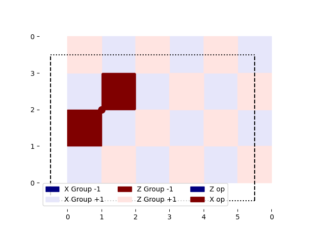
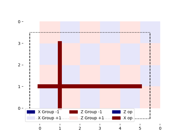
With this function, we can quickly view the expectation values and the location of the additional X operation. The operation changes the expectation values for the adjacent Z groups.

fig, ax = excitation_plot(x_expvals, z_expvals)
ax.scatter(*zip(*single_x), color="maroon", s=100)
plt.show()

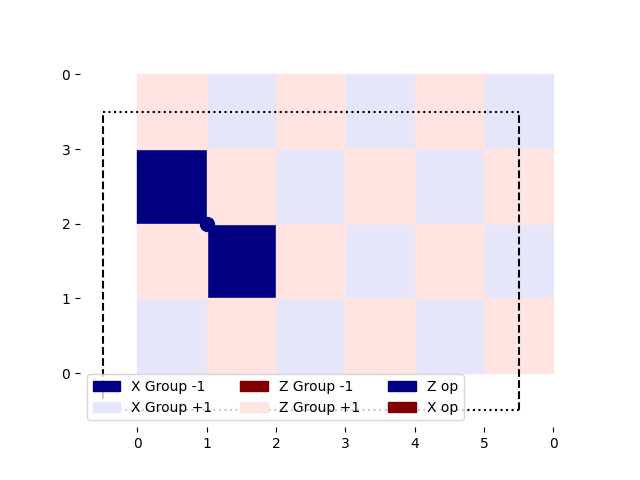
What if we apply a Z operation instead at the same site? We instead get two X Group excitations.

single_z = [(1, 2)]

expvals = excitations([], single_z)
x_expvals, z_expvals = separate_expvals(expvals)
print_info(x_expvals, z_expvals)

Out:

Total energy:  -19.999999999999996
Energy above the ground state:  4.0
X Group occupation numbers:  [0.0, 1.0, 1.0, 0.0, 0.0, 0.0, 0.0, 0.0, 0.0, 0.0, 0.0, 0.0]
Z Group occupation numbers:  [0.0, 0.0, 0.0, 0.0, 0.0, 0.0, 0.0, 0.0, 0.0, 0.0, 0.0, 0.0]

fig, ax = excitation_plot(x_expvals, z_expvals)
ax.scatter(*zip(*single_z), color="navy", s=100)
plt.show()

What happens if we apply the same perturbation twice at one location? We regain the ground state.

The excitations of the toric code are Majorana particles: particles that are their own antiparticles. While postulated to exist in standard particle physics, Majorana particles have only been experimentally seen as quasiparticle excitations in materials.

We can think of the second operation as creating another set of excitations at the same location. This second pair then annihilates the existing particles.

single_z = [(1, 2)]

expvals = excitations([], single_z + single_z)
x_expvals, z_expvals = separate_expvals(expvals)

print_info(x_expvals, z_expvals)

Out:

Total energy:  -23.999999999999996
Energy above the ground state:  0.0
X Group occupation numbers:  [0.0, 0.0, 0.0, 0.0, 0.0, 0.0, 0.0, 0.0, 0.0, 0.0, 0.0, 0.0]
Z Group occupation numbers:  [0.0, 0.0, 0.0, 0.0, 0.0, 0.0, 0.0, 0.0, 0.0, 0.0, 0.0, 0.0]

Moving Excitations and String Operators

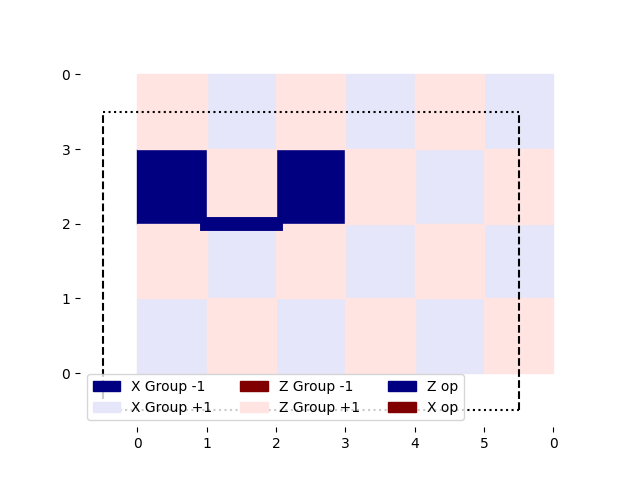
What if we create a second set of particles such that one of the new particles overlaps with an existing particle? One old and one new particle annihilate each other. One old and one new particle remain. We still have two particles in total.

Alternatively, we can view the second operation as moving a single excitation.

Let’s see what that looks like in code:

two_z = [(1, 2), (2, 2)]

expvals = excitations([], two_z)
x_expvals, z_expvals = separate_expvals(expvals)

print_info(x_expvals, z_expvals)

Out:

Total energy:  -19.999999999999996
Energy above the ground state:  4.0
X Group occupation numbers:  [0.0, 0.0, 1.0, 0.0, 0.0, 0.0, 1.0, 0.0, 0.0, 0.0, 0.0, 0.0]
Z Group occupation numbers:  [0.0, 0.0, 0.0, 0.0, 0.0, 0.0, 0.0, 0.0, 0.0, 0.0, 0.0, 0.0]

fig, ax = excitation_plot(x_expvals, z_expvals)
ax.plot(*zip(*two_z), color="navy", linewidth=10)
plt.show()

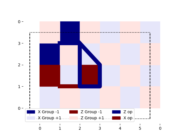
In that example, we just moved an excitation a little. How about we try moving it even further?

long_string = [(1, 2), (2, 2), (3, 2), (4, 1)]

expvals = excitations([], long_string)
x_expvals, z_expvals = separate_expvals(expvals)

print_info(x_expvals, z_expvals)

Out:

Total energy:  -19.999999999999996
Energy above the ground state:  4.0
X Group occupation numbers:  [0.0, 0.0, 1.0, 0.0, 0.0, 0.0, 0.0, 0.0, 1.0, 0.0, 0.0, 0.0]
Z Group occupation numbers:  [0.0, 0.0, 0.0, 0.0, 0.0, 0.0, 0.0, 0.0, 0.0, 0.0, 0.0, 0.0]

fig, ax = excitation_plot(x_expvals, z_expvals)
ax.plot(*zip(*long_string), color="navy", linewidth=10)
plt.show()

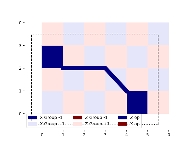
We end up with strings of operations that connect pairs of quasiparticles.

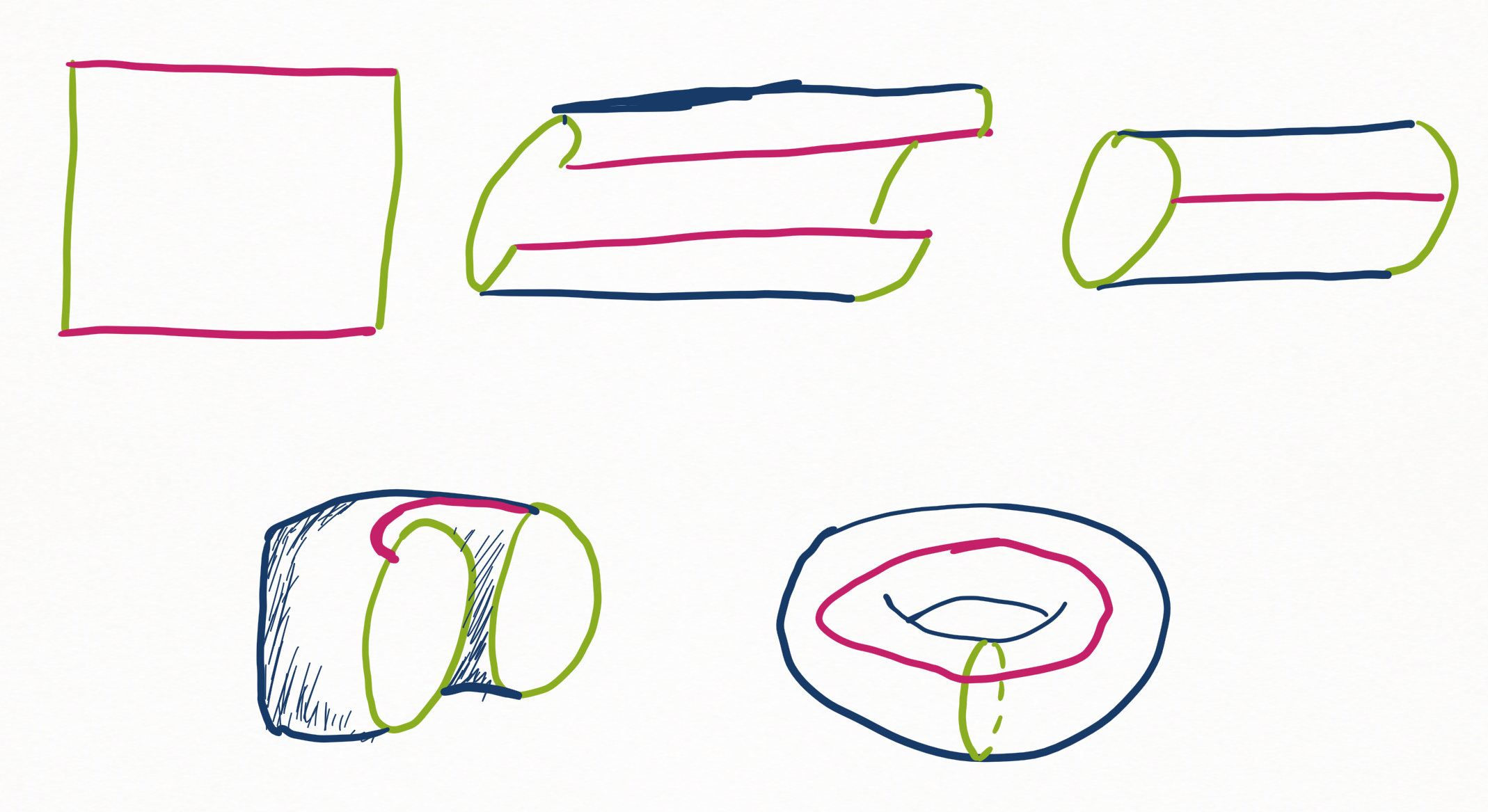
We can use a branch of topology called Homotopy to describe the relationship between these strings and the wave function. Two paths \(s_1\) and \(s_2\) are homotopy equivalent or homotopic if they can be continuously deformed into each other:

\[s_1 \sim s_2\]

In the following picture, assume the red “X” is a defect in space, like a tear in a sheet. The two blue paths are equivalent because you can smoothly move one into the other. You cannot move the blue path into the green path without going through the defect, so they are not equivalent to each other.

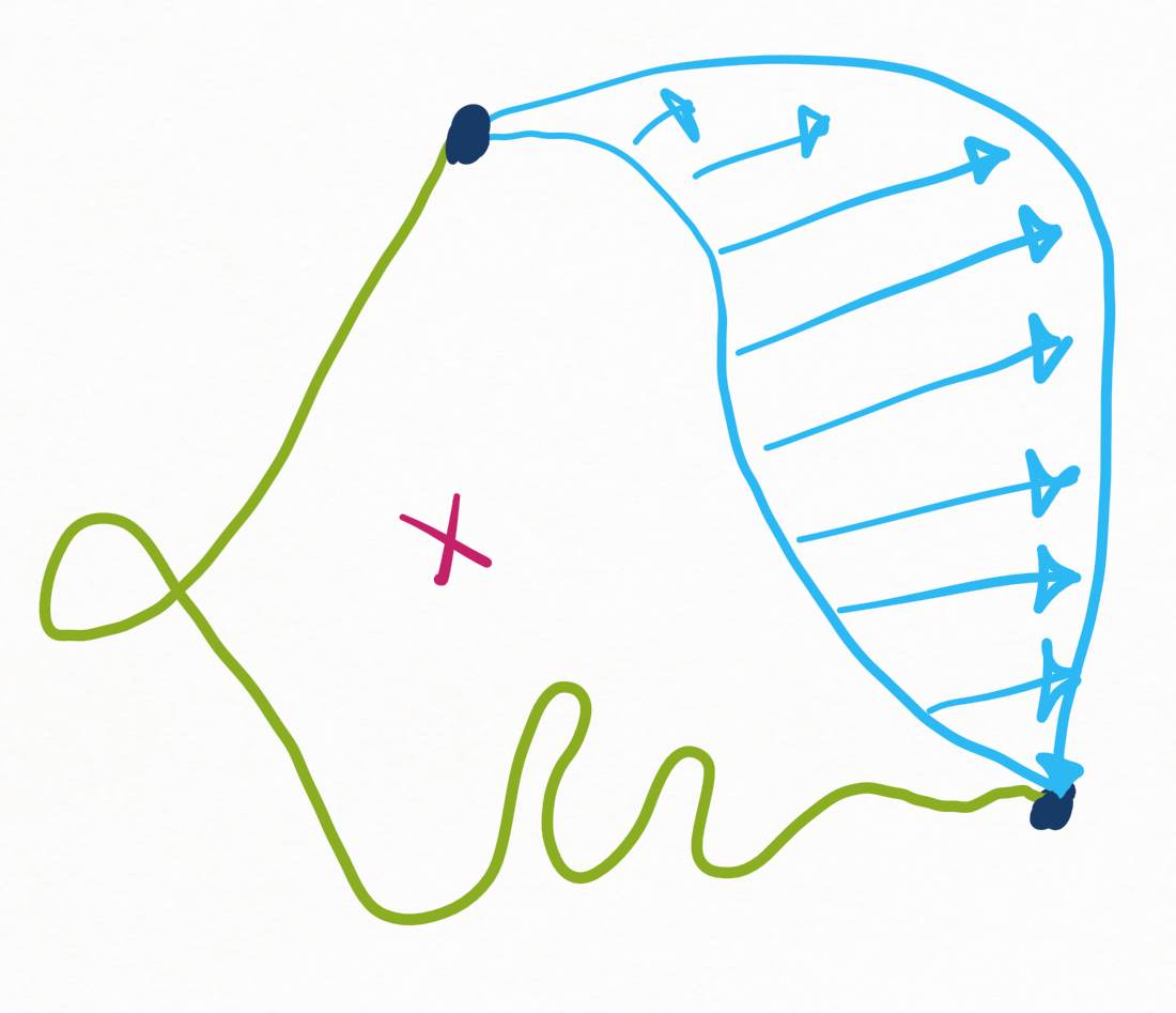
Paths are homotopy equivalent if they can be smoothly deformed into each other.

We can divide the set of all possible paths into homotopy classes. A homotopy class is an equivalence class under homotopy. Every member of the same homotopy class can be deformed into every other member of the same class, and members of different homotopy classes cannot be deformed into each other. All the homotopy classes for a given space \(S\) form its first homotopy group, denoted by \(\pi_1(S)\). The first homotopy group of a space is also called its fundamental group.

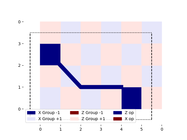
How do these mathematical concepts apply to the toric code model? To find out, let’s look at a string of Z operations homotopic to the one above.

This next string creates the same final state. Only the homotopy class of the path used to create the excitations influences the occupation numbers and total energy. If the endpoints are the same and the path doesn’t wrap around the torus or other particles, the details do not impact any observables.

equivalent_string = [(1, 2), (2, 1), (3, 1), (4, 1)]

expvals = excitations([], equivalent_string)
x_expvals, z_expvals = separate_expvals(expvals)

print_info(x_expvals, z_expvals)

Out:

Total energy:  -19.999999999999996
Energy above the ground state:  4.0
X Group occupation numbers:  [0.0, 0.0, 1.0, 0.0, 0.0, 0.0, 0.0, 0.0, 1.0, 0.0, 0.0, 0.0]
Z Group occupation numbers:  [0.0, 0.0, 0.0, 0.0, 0.0, 0.0, 0.0, 0.0, 0.0, 0.0, 0.0, 0.0]

fig, ax = excitation_plot(x_expvals, z_expvals)
ax.plot(*zip(*equivalent_string), color="navy", linewidth=10)
plt.show()

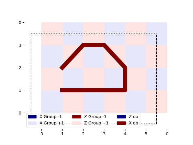
Contractible loops

We can also have a loop of operations that doesn’t create any new excitations. The loop forms a pair, moves one around in a circle, and then annihilates the two particles again.

contractible_loop = [(1, 1), (2, 1), (3, 1), (4, 1), (4, 2), (3, 3), (2, 3), (1, 2)]

expvals = excitations(contractible_loop, [])
x_expvals, z_expvals = separate_expvals(expvals)
print_info(x_expvals, z_expvals)

Out:

Total energy:  -23.999999999999996
Energy above the ground state:  0.0
X Group occupation numbers:  [0.0, 0.0, 0.0, 0.0, 0.0, 0.0, 0.0, 0.0, 0.0, 0.0, 0.0, 0.0]
Z Group occupation numbers:  [0.0, 0.0, 0.0, 0.0, 0.0, 0.0, 0.0, 0.0, 0.0, 0.0, 0.0, 0.0]

fig, ax = excitation_plot(x_expvals, z_expvals)

ax.plot(*zip(*contractible_loop), color="maroon", linewidth=10)

plt.show()

The loop doesn’t affect the positions of any excitations, but does it affect the state at all?

We will look at the probabilities instead of the expectation values to answer that question.

@qml.qnode(dev, diff_method=None)
def probs(x_sites, z_sites):
    state_prep()

    for s in x_sites:
        qml.PauliX(Wire(*s))

    for s in z_sites:
        qml.PauliZ(Wire(*s))

    return qml.probs(wires=[Wire(*s) for s in all_sites])


null_probs = probs([], [])
contractible_probs = probs(contractible_loop, [])

print("Are the probabilities equal? ", np.allclose(null_probs, contractible_probs))

Out:

Are the probabilities equal?  True

The toric code’s dependence on the homotopy of the path explains this result. All paths we can smoothly deform into each other will give the same result. The contractible loop can be smoothly deformed to nothing, so the state with the contractible loop is the same as the state with no loop, our initial \(|G\rangle\).

Looping the torus

On the torus, we have four types of unique paths:

• The trivial path that contracts to nothing

• A horizontal loop around the boundaries

• A vertical loop around the boundaries

• A loop around both the horizontal and vertical boundaries

The homotopy group of a torus can be generated by a horizontal loop and a vertical loop around the boundaries.

Each of these paths represents a member of the first homotopy group of the torus: \(\pi_1(T) = \mathbb{Z}^2\) modulo 2.

None of these loops of X operations create net excitations, so the wave function remains in the ground state.

horizontal_loop = [(i, 1) for i in range(width)]
vertical_loop = [(1, i) for i in range(height)]

expvals = excitations(horizontal_loop + vertical_loop, [])
fig, ax = excitation_plot(*separate_expvals(expvals))

ax.plot(*zip(*horizontal_loop), color="maroon", linewidth=10)
ax.plot(*zip(*vertical_loop), color="maroon", linewidth=10)

plt.show()

We can compute the probabilities for each of these four types of loops:

null_probs = probs([], [])
horizontal_probs = probs(horizontal_loop, [])
vertical_probs = probs(vertical_loop, [])
combo_probs = probs(horizontal_loop + vertical_loop, [])

While X and Z operations can change the group operator expectation values and create quasiparticles, only X operators can change the probability distribution. Applying a Z operator would only rotate the phase of the state and not change any amplitudes. Hence we only use loops of X operators in this section. I encourage you to try this analysis with loops of Z operators to confirm that they do not change the probability distribution.

We can compare the original state and one with a horizontal loop to see if the probability distributions are different:

print("Are the probabilities equal? ", qml.math.allclose(null_probs, horizontal_probs))
print("Is this significant?")
print("Maximum difference in probabilities: ", max(abs(null_probs - horizontal_probs)))
print("Maximum probability: ", max(null_probs))

Out:

Are the probabilities equal?  False
Is this significant?
Maximum difference in probabilities:  0.00048828124999999913
Maximum probability:  0.00048828124999999913

These numbers seem small, but remember we have 24 qubits, and thus \(2^{24}=16777216\) probability components. Since the maximum difference in probabilities is the same size as the maximum probability, we know this isn’t just random fluctuations and errors. The states are different, but the energies are the same, so they are degenerate.

That compared a horizontal “x” loop with the initial ground state. How about the other two types of loops? Let’s iterate over all combinations of two probability distributions to see if any match.

probs_type_labels = ["null", "x", "y", "combo"]
all_probs = [null_probs, horizontal_probs, vertical_probs, combo_probs]

print("\t" + "\t".join(probs_type_labels))

for name, probs1 in zip(probs_type_labels, all_probs):
    comparisons = (str(np.allclose(probs1, probs2)) for probs2 in all_probs)
    print(name, "\t", "\t".join(comparisons))

Out:

        null    x       y       combo
null     True   False   False   False
x        False  True    False   False
y        False  False   True    False
combo    False  False   False   True

This table shows the model has four distinct ground states. More importantly, these ground states are separated from each other by long-range operations. We must perform a loop of operations across the entire lattice to switch between degenerate ground states.

This four-way degeneracy is the source of the error correction in the toric code. Instead of 24 qubits, we work with two logical qubits (4 states) that are well separated from each other by topological operations.

Note

I encourage dedicated readers to explore what happens when a path loops the same boundaries twice.

In this section, we’ve seen that the space of ground states is directly related to the first homotopy group of the lattice. The first homotopy group of a torus is \(\pi_1(T) = \mathbb{Z}^2\), and the space of ground states is that group modulo two, \(\mathbb{Z}_2^2\).

What if we defined the model on a differently shaped lattice? Then the space of the ground state would change to reflect the first homotopy group of that space. For example, if the model was defined on a sphere, then only a single unique ground state would exist. Adding defects like missing sites to the lattice also changes the topology. Error correction with the toric code often uses missing sites to add additional logical qubits.

Mutual and Exchange Statistics

The hole in the center of the donut isn’t the only thing that prevents paths from smoothly deforming into each other. We don’t yet know if we can distort paths past other particles.

When one indistinguishable fermion of spin 1/2 orbits another fermion of the same type, the combined wave function picks up a relative phase of negative one. When fermions of different types orbit each other, the state is unchanged. For example, if an electron goes around a proton and returns to the same spot, the wave function is unchanged. If a boson orbits around a different type of boson, again, the wave function is unchanged.

What if a particle went around a different type of particle and everything picked up a phase? Would it be a boson or a fermion?

It would be something else entirely: an anyon. An anyon is anything that doesn’t cleanly fall into the boson/fermion categorization of particles.

While the toric code is just an extremely useful mathematical model, anyons exist in physical materials. For example, fractional quantum Hall systems have anyonic particles with spin \(1/q\) for different integers \(q\).

The statistics are described by the phase accumulated by moving one particle around another. For example, if the particle picks up phases like a fermion, then it obeys Fermi-Dirac statistics. Exchange statistics are described by the phases that accumulate from exchanging the same type of particles. Mutual statistics are characterized by the phase acquired by moving one particle around a particle of a different type.

To measure the mutual statistics of a Z Group excitation and an X group excitation, we need to prepare at least one of each type of particle and then orbit one around the other.

The following code rotates an X Group excitation around a Z Group excitation.

prep1 = [(1, 1), (2, 1)]
prep2 = [(1, 3)]
loop1 = [(2, 3), (2, 2), (2, 1), (3, 1), (3, 2), (2, 3)]

expvals = excitations(prep1, prep2 + loop1)
x_expvals, z_expvals = separate_expvals(expvals)

fig, ax = excitation_plot(x_expvals, z_expvals)

ax.plot(*zip(*prep1), color="maroon", linewidth=10)
ax.plot(*zip(*(prep2 + loop1)), color="navy", linewidth=10)

plt.show()

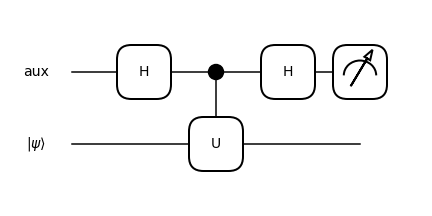
While we managed to loop one particle around the other, we did not extract the relative phase applied to the wave function. To procure this information, we will need the Hadamard test.

Hadamard test

The Hadamard test extracts the real component of a unitary operation \(\text{Re}\left(\langle \psi | U | \psi \rangle \right)\). If the unitary operation just applies a phase \(U |\psi\rangle = e^{i \phi} |\psi \rangle\), the measured quantity reduces to \(\cos (\phi)\).

The steps in the Hadamard test are:

1. Prepare the auxiliary qubit into a superposition with a Hadamard gate

2. Apply a controlled version of the operation with the auxiliary qubit as the control

3. Apply another Hadamard gate to the auxiliary qubit

4. Measure the auxiliary qubit in the Z-basis

Note

For extra understanding, validate the Hadamard test algorithm using pen and paper.

Below we implement this algorithm in PennyLane and measure the mutual exchange statistics of an X Group excitation and a Z Group excitation.

dev_aux = qml.device("lightning.qubit", wires=[Wire(*s) for s in all_sites] + ["aux"])

def loop(x_loop, z_loop):
    for s in x_loop:
        qml.PauliX(Wire(*s))
    for s in z_loop:
        qml.PauliZ(Wire(*s))

@qml.qnode(dev_aux, diff_method=None)
def hadamard_test(x_prep, z_prep, x_loop, z_loop):
    state_prep()

    for s in x_prep:
        qml.PauliX(Wire(*s))

    for s in z_prep:
        qml.PauliZ(Wire(*s))

    qml.Hadamard("aux")
    qml.ctrl(loop, control="aux")(x_loop, z_loop)
    qml.Hadamard("aux")
    return qml.expval(qml.PauliZ("aux"))

x_around_z = hadamard_test(prep1, prep2, [], loop1)
print("Move x excitation around z excitation: ", x_around_z)

Out:

Move x excitation around z excitation:  -0.9999999999999991

We just moved two different types of particles around each other and picked up a phase. As neither bosons nor fermions behave like this, this result demonstrates that the excitations of a toric code are anyons.

Note

I encourage dedicated readers to calculate the phase accumulated by exchanging:

• A Z Group excitation and a Z Group Excitation

• An X Group excitation and an X Group Excitation

• A combination \(\Psi\) particle and an X Group excitation

• A combination \(\Psi\) particle and a Z Group excitation

• A combination \(\Psi\) particle with another \(\Psi\) particle

The combination particle should behave like a standard fermion. You can create and move combination particles by applying PauliY operations.

In this demo, we have demonstrated:

1. How to prepare the ground state of the toric code model on a lattice of qubits

2. How to create and move excitations

3. The ground state degeneracy of the model on a toric lattice, arising from homotopically distinct loops of operations

4. The excitations are anyons due to non-trivial mutual statistics Make sure to go and modify the code as suggested if you wish to gain more intuition.

Do check the references below if you want to learn more!

References

1(1,2)

Kitaev, A. Yu. “Fault-tolerant quantum computation by anyons.” Annals of Physics 303.1 (2003): 2-30.. (arXiv)

2

Fowler, Austin G., et al. “Surface codes: Towards practical large-scale quantum computation.” Physical Review A 86.3 (2012): 032324.. (arXiv)

3

Satzinger, K. J., et al. “Realizing topologically ordered states on a quantum processor.” Science 374.6572 (2021): 1237-1241.. (arXiv)

4

Savary, Lucile, and Leon Balents. “Quantum spin liquids: a review.” Reports on Progress in Physics 80.1 (2016): 016502.. (arXiv)

5

Araujo de Resende, M. F. “A pedagogical overview on 2D and 3D Toric Codes and the origin of their topological orders.” Reviews in Mathematical Physics 32.02 (2020): 2030002. (arXiv)

About the author

Christina Lee

Christina is currently a quantum software developer at Xanadu working on PennyLane. Outside of coding, she enjoys running, yoga, and piano.

demos/tutorial_toric_code

 

Download Python script

 

Download Notebook

 

View on GitHub