Variational Quantum Thermalizer

Author: Jack Ceroni — Posted: 7 July 2020. Last updated: 28 January 2021.

This demonstration discusses theory and experiments relating to a recently proposed quantum algorithm called the Variational Quantum Thermalizer (VQT): a generalization of the well-know Variational Quantum Eigensolver (VQE) to systems with non-zero temperatures.

The Idea

The goal of the VQT is to prepare the thermal state of a given Hamiltonian \(\hat{H}\) at temperature \(T\), which is defined as

\[\rho_\text{thermal} \ = \ \frac{e^{- \hat{H} \beta}}{\text{Tr}(e^{- \hat{H} \beta})} \ = \ \frac{e^{- \hat{H} \beta}}{Z_{\beta}},\]

where \(\beta \ = \ 1/T\). The thermal state is a mixed state, which means that can be described by an ensemble of pure states. Since we are attempting to learn a mixed state, we must deviate from the standard variational method of passing a pure state through an ansatz circuit, and minimizing the energy expectation.

The VQT begins with an initial density matrix, \(\rho_{\theta}\), described by a probability distribution parametrized by some collection of parameters \(\theta\), and an ensemble of pure states, \(\{|\psi_i\rangle\}\). Let \(p_i(\theta_i)\) be the probability corresponding to the \(i\)-th pure state. We sample from this probability distribution to get some pure state \(|\psi_k\rangle\), which we pass through a parametrized circuit, \(U(\phi)\). From the results of this circuit, we then calculate \(\langle \psi_k | U^{\dagger}(\phi) \hat{H}\, U(\phi) |\psi_k\rangle\). Repeating this process multiple times and taking the average of these expectation values gives us the the expectation value of \(\hat{H}\) with respect to \(U \rho_{\theta} U^{\dagger}\).

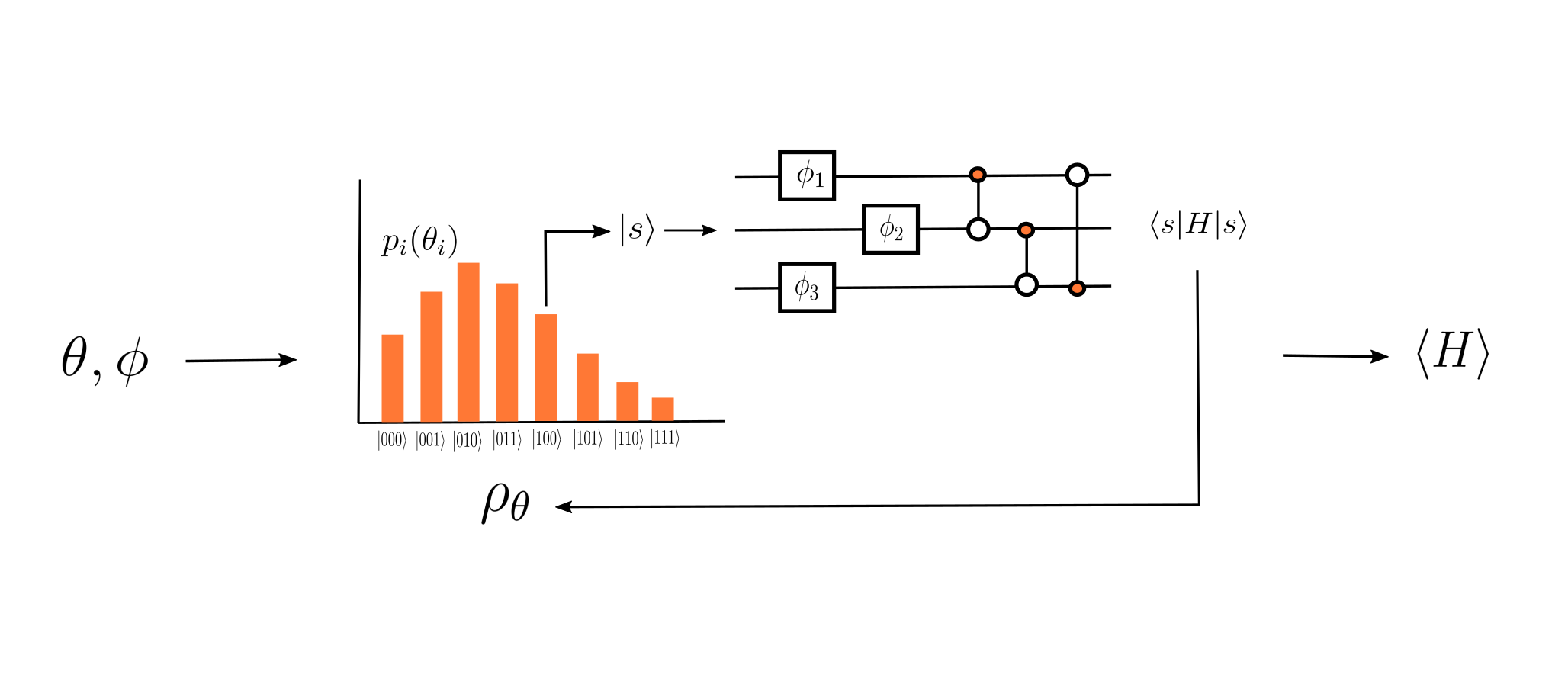
Inputted parameters create an initial density matrix and a parametrized ansatz, which are used to calculate the expectation value of the Hamiltonian with respect to a new mixed state.

Arguably, the most important part of a variational circuit is its cost function, which we attempt to minimize with a classical optimizer. In VQE, we generally try to minimize \(\langle \psi(\theta) | \hat{H} | \psi(\theta) \rangle\) which, upon minimization, gives us a parametrized circuit that prepares a good approximation to the ground state of \(\hat{H}\). In the VQT, the goal is to arrive at a parametrized probability distribution, and a parametrized ansatz, that generate a good approximation to the thermal state. This generally involves more than calculating the energy expectation value. Luckily, we know that the thermal state of \(\hat{H}\) minimizes the following free-energy cost function

\[\mathcal{L}(\theta, \ \phi) \ = \ \beta \ \text{Tr}( \hat{H} \ \hat{U}(\phi) \rho_{\theta} \hat{U}(\phi)^{\dagger} ) \ - \ S_\theta,\]

where \(S_{\theta}\) is the von Neumann entropy of \(U \rho_{\theta} U^{\dagger}\), which is the same as the von Neumann entropy of \(\rho_{\theta}\) due to invariance of entropy under unitary transformations. This cost function is minimized when \(\hat{U}(\phi) \rho_{\theta} \hat{U}(\phi)^{\dagger} \ = \ \rho_{\text{thermal}}\), so similarly to VQE, we minimize it with a classical optimizer to obtain the target parameters, and thus the target state.

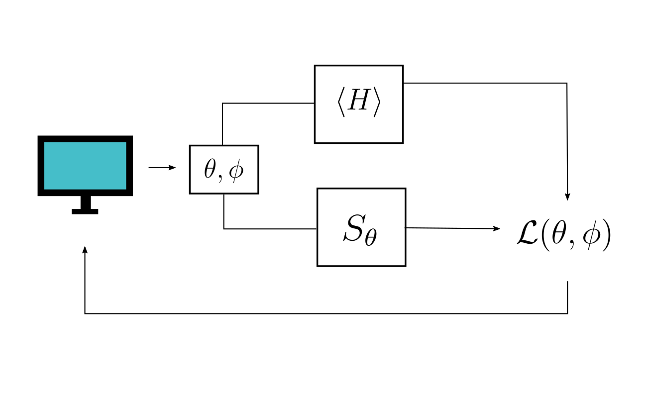
A high-level representation of how the VQT works.

All together, the outlined processes give us a general protocol to generate thermal states.

Simulating the VQT for a 4-Qubit Heisenberg Model

In this demonstration, we simulate the 4-qubit Heisenberg model. We can begin by importing the necessary dependencies.

import pennylane as qml
from matplotlib import pyplot as plt
import numpy as np
from numpy import array
import scipy
from scipy.optimize import minimize
import networkx as nx
import seaborn
import itertools

np.random.seed(42)

The Heisenberg Hamiltonian is defined as

\[\hat{H} \ = \ \displaystyle\sum_{(i, j) \in E} X_i X_j \ + \ Z_i Z_j \ + \ Y_i Y_j,\]

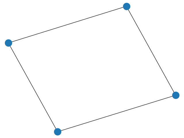
where \(X_i\), \(Y_i\) and \(Z_i\) are the Pauli gates acting on the \(i\)-th qubit. In addition, \(E\) is the set of edges in the graph \(G \ = \ (V, \ E)\) describing the interactions between the qubits. In this demonstration, we define the interaction graph to be the cycle graph:

interaction_graph = nx.cycle_graph(4)
nx.draw(interaction_graph)

With this, we can calculate the matrix representation of the Heisenberg Hamiltonian in the computational basis:

def create_hamiltonian_matrix(n, graph):

    matrix = np.zeros((2 ** n, 2 ** n))

    for i in graph.edges:
        x = y = z = 1
        for j in range(0, n):
            if j == i[0] or j == i[1]:
                x = np.kron(x, qml.matrix(qml.PauliX)(0))
                y = np.kron(y, qml.matrix(qml.PauliY)(0))
                z = np.kron(z, qml.matrix(qml.PauliZ)(0))
            else:
                x = np.kron(x, np.identity(2))
                y = np.kron(y, np.identity(2))
                z = np.kron(z, np.identity(2))

        matrix = np.add(matrix, np.add(x, np.add(y, z)))

    return matrix


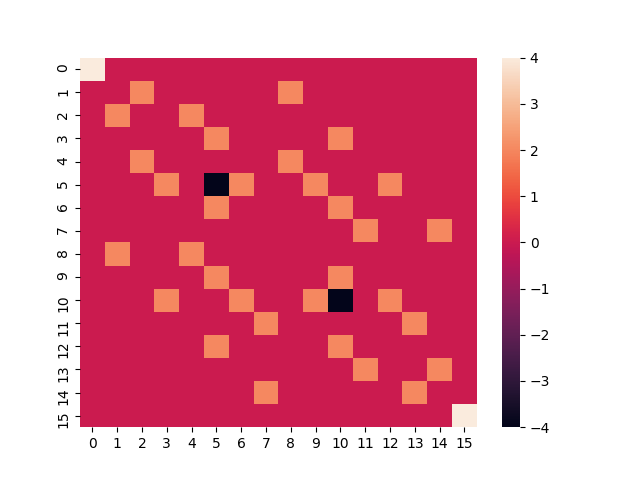
ham_matrix = create_hamiltonian_matrix(4, interaction_graph)

# Prints a visual representation of the Hamiltonian matrix
seaborn.heatmap(ham_matrix.real)
plt.show()

With this done, we construct the VQT. We begin by defining some fixed variables that are used throughout the simulation:

beta = 2  # beta = 1/T
nr_qubits = 4

The first step of the VQT is to create the initial density matrix, \(\rho_\theta\). In this demonstration, we let \(\rho_\theta\) be factorized, meaning that it can be written as an uncorrelated tensor product of \(4\) one-qubit density matrices that are diagonal in the computational basis. The motivation is that in this factorized model, the number of \(\theta_i\) parameters needed to describe \(\rho_\theta\) scales linearly rather than exponentially with the number of qubits. For each one-qubit system described by \(\rho_\theta^i\), we have

\[\rho_{\theta}^{i} \ = \ p_i(\theta_i) |0\rangle \langle 0| \ + \ (1 \ - \ p_i(\theta_i))|1\rangle \langle1|.\]

From here, all we have to do is define \(p_i(\theta_i)\), which we choose to be the sigmoid

\[p_{i}(\theta_{i}) \ = \ \frac{e^{\theta_i}}{e^{\theta_i} \ + \ 1}.\]

def sigmoid(x):
    return np.exp(x) / (np.exp(x) + 1)

This is a natural choice for probability function, as it has a range of \([0, \ 1]\), meaning that we don’t need to restrict the domain of \(\theta_i\) to some subset of the real numbers. With the probability function defined, we can write a method that gives us the diagonal elements of each one-qubit density matrix, for some parameters \(\theta\):

def prob_dist(params):
    return np.vstack([sigmoid(params), 1 - sigmoid(params)]).T

Creating the Ansatz Circuit

With this done, we can move on to defining the ansatz circuit, \(U(\phi)\), composed of rotational and coupling layers. The rotation layer is simply RX, RY, and RZ gates applied to each qubit. We make use of the AngleEmbedding function, which allows us to easily pass parameters into rotational layers.

def single_rotation(phi_params, qubits):

    rotations = ["Z", "Y", "X"]
    for i in range(0, len(rotations)):
        qml.AngleEmbedding(phi_params[i], wires=qubits, rotation=rotations[i])

To construct the general ansatz, we combine the method we have just defined with a collection of parametrized coupling gates placed between qubits that share an edge in the interaction graph. In addition, we define the depth of the ansatz, and the device on which the simulations are run:

depth = 4
dev = qml.device("default.qubit", wires=nr_qubits)


def quantum_circuit(rotation_params, coupling_params, sample=None):

    # Prepares the initial basis state corresponding to the sample
    qml.BasisStatePreparation(sample, wires=range(nr_qubits))

    # Prepares the variational ansatz for the circuit
    for i in range(0, depth):
        single_rotation(rotation_params[i], range(nr_qubits))
        qml.broadcast(
            unitary=qml.CRX,
            pattern="ring",
            wires=range(nr_qubits),
            parameters=coupling_params[i]
        )

    # Calculates the expectation value of the Hamiltonian with respect to the prepared states
    return qml.expval(qml.Hermitian(ham_matrix, wires=range(nr_qubits)))


# Constructs the QNode
qnode = qml.QNode(quantum_circuit, dev, interface="autograd")

We can get an idea of what this circuit looks like by printing out a test circuit:

rotation_params = [[[1, 1, 1, 1], [1, 1, 1, 1], [1, 1, 1, 1]] for i in range(0, depth)]
coupling_params = [[1, 1, 1, 1] for i in range(0, depth)]
print(qml.draw(qnode, expansion_strategy="device", show_matrices=True)(rotation_params, coupling_params, sample=[1, 0, 1, 0]))

Out:

0: ──X─────────RZ(1.00)──RY(1.00)──RX(1.00)─╭●────────────────────────────╭RX(1.00)──RZ(1.00)
1: ──RZ(1.00)──RY(1.00)──RX(1.00)───────────╰RX(1.00)─╭●──────────────────│──────────RZ(1.00)
2: ──X─────────RZ(1.00)──RY(1.00)──RX(1.00)───────────╰RX(1.00)─╭●────────│──────────RZ(1.00)
3: ──RZ(1.00)──RY(1.00)──RX(1.00)───────────────────────────────╰RX(1.00)─╰●─────────RZ(1.00)

───RY(1.00)──RX(1.00)─╭●────────────────────────────╭RX(1.00)──RZ(1.00)──RY(1.00)──RX(1.00)
───RY(1.00)──RX(1.00)─╰RX(1.00)─╭●──────────────────│──────────RZ(1.00)──RY(1.00)──RX(1.00)
───RY(1.00)──RX(1.00)───────────╰RX(1.00)─╭●────────│──────────RZ(1.00)──RY(1.00)──RX(1.00)
───RY(1.00)──RX(1.00)─────────────────────╰RX(1.00)─╰●─────────RZ(1.00)──RY(1.00)──RX(1.00)

──╭●────────────────────────────╭RX(1.00)──RZ(1.00)──RY(1.00)──RX(1.00)─╭●─────────────────
──╰RX(1.00)─╭●──────────────────│──────────RZ(1.00)──RY(1.00)──RX(1.00)─╰RX(1.00)─╭●───────
────────────╰RX(1.00)─╭●────────│──────────RZ(1.00)──RY(1.00)──RX(1.00)───────────╰RX(1.00)
──────────────────────╰RX(1.00)─╰●─────────RZ(1.00)──RY(1.00)──RX(1.00)────────────────────

────────────╭RX(1.00)─┤ ╭<𝓗(M0)>
────────────│─────────┤ ├<𝓗(M0)>
──╭●────────│─────────┤ ├<𝓗(M0)>
──╰RX(1.00)─╰●────────┤ ╰<𝓗(M0)>
M0 =
[[ 4.+0.j  0.+0.j  0.+0.j  0.+0.j  0.+0.j  0.+0.j  0.+0.j  0.+0.j  0.+0.j
   0.+0.j  0.+0.j  0.+0.j  0.+0.j  0.+0.j  0.+0.j  0.+0.j]
 [ 0.+0.j  0.+0.j  2.+0.j  0.+0.j  0.+0.j  0.+0.j  0.+0.j  0.+0.j  2.+0.j
   0.+0.j  0.+0.j  0.+0.j  0.+0.j  0.+0.j  0.+0.j  0.+0.j]
 [ 0.+0.j  2.+0.j  0.+0.j  0.+0.j  2.+0.j  0.+0.j  0.+0.j  0.+0.j  0.+0.j
   0.+0.j  0.+0.j  0.+0.j  0.+0.j  0.+0.j  0.+0.j  0.+0.j]
 [ 0.+0.j  0.+0.j  0.+0.j  0.+0.j  0.+0.j  2.+0.j  0.+0.j  0.+0.j  0.+0.j
   0.+0.j  2.+0.j  0.+0.j  0.+0.j  0.+0.j  0.+0.j  0.+0.j]
 [ 0.+0.j  0.+0.j  2.+0.j  0.+0.j  0.+0.j  0.+0.j  0.+0.j  0.+0.j  2.+0.j
   0.+0.j  0.+0.j  0.+0.j  0.+0.j  0.+0.j  0.+0.j  0.+0.j]
 [ 0.+0.j  0.+0.j  0.+0.j  2.+0.j  0.+0.j -4.+0.j  2.+0.j  0.+0.j  0.+0.j
   2.+0.j  0.+0.j  0.+0.j  2.+0.j  0.+0.j  0.+0.j  0.+0.j]
 [ 0.+0.j  0.+0.j  0.+0.j  0.+0.j  0.+0.j  2.+0.j  0.+0.j  0.+0.j  0.+0.j
   0.+0.j  2.+0.j  0.+0.j  0.+0.j  0.+0.j  0.+0.j  0.+0.j]
 [ 0.+0.j  0.+0.j  0.+0.j  0.+0.j  0.+0.j  0.+0.j  0.+0.j  0.+0.j  0.+0.j
   0.+0.j  0.+0.j  2.+0.j  0.+0.j  0.+0.j  2.+0.j  0.+0.j]
 [ 0.+0.j  2.+0.j  0.+0.j  0.+0.j  2.+0.j  0.+0.j  0.+0.j  0.+0.j  0.+0.j
   0.+0.j  0.+0.j  0.+0.j  0.+0.j  0.+0.j  0.+0.j  0.+0.j]
 [ 0.+0.j  0.+0.j  0.+0.j  0.+0.j  0.+0.j  2.+0.j  0.+0.j  0.+0.j  0.+0.j
   0.+0.j  2.+0.j  0.+0.j  0.+0.j  0.+0.j  0.+0.j  0.+0.j]
 [ 0.+0.j  0.+0.j  0.+0.j  2.+0.j  0.+0.j  0.+0.j  2.+0.j  0.+0.j  0.+0.j
   2.+0.j -4.+0.j  0.+0.j  2.+0.j  0.+0.j  0.+0.j  0.+0.j]
 [ 0.+0.j  0.+0.j  0.+0.j  0.+0.j  0.+0.j  0.+0.j  0.+0.j  2.+0.j  0.+0.j
   0.+0.j  0.+0.j  0.+0.j  0.+0.j  2.+0.j  0.+0.j  0.+0.j]
 [ 0.+0.j  0.+0.j  0.+0.j  0.+0.j  0.+0.j  2.+0.j  0.+0.j  0.+0.j  0.+0.j
   0.+0.j  2.+0.j  0.+0.j  0.+0.j  0.+0.j  0.+0.j  0.+0.j]
 [ 0.+0.j  0.+0.j  0.+0.j  0.+0.j  0.+0.j  0.+0.j  0.+0.j  0.+0.j  0.+0.j
   0.+0.j  0.+0.j  2.+0.j  0.+0.j  0.+0.j  2.+0.j  0.+0.j]
 [ 0.+0.j  0.+0.j  0.+0.j  0.+0.j  0.+0.j  0.+0.j  0.+0.j  2.+0.j  0.+0.j
   0.+0.j  0.+0.j  0.+0.j  0.+0.j  2.+0.j  0.+0.j  0.+0.j]
 [ 0.+0.j  0.+0.j  0.+0.j  0.+0.j  0.+0.j  0.+0.j  0.+0.j  0.+0.j  0.+0.j
   0.+0.j  0.+0.j  0.+0.j  0.+0.j  0.+0.j  0.+0.j  4.+0.j]]

Recall that the final cost function depends not only on the expectation value of the Hamiltonian, but also the von Neumann entropy of the state, which is determined by the collection of \(p_i(\theta_i)\)s. Since the entropy of a collection of multiple uncorrelated subsystems is the same as the sum of the individual values of entropy for each subsystem, we can sum the entropy values of each one-qubit system in the factorized space to get the total:

def calculate_entropy(distribution):

    total_entropy = 0
    for d in distribution:
        total_entropy += -1 * d[0] * np.log(d[0]) + -1 * d[1] * np.log(d[1])

    # Returns an array of the entropy values of the different initial density matrices

    return total_entropy

The Cost Function

Finally, we combine the ansatz and the entropy function to get the cost function. In this demonstration, we deviate slightly from how VQT would be performed in practice. Instead of sampling from the probability distribution describing the initial mixed state, we use the ansatz to calculate \(\langle x_i | U^{\dagger}(\phi) \hat{H} \,U(\phi) |x_i\rangle\) for each basis state \(|x_i\rangle\). We then multiply each of these expectation values by their corresponding \((\rho_\theta)_{ii}\), which is exactly the probability of sampling \(|x_i\rangle\) from the distribution. Summing each of these terms together gives us the expected value of the Hamiltonian with respect to the transformed density matrix.

In the case of this small, simple model, exact calculations such as this reduce the number of circuit executions, and thus the total execution time.

You may have noticed previously that the “structure” of the parameters list passed into the ansatz is quite complicated. We write a general function that takes a one-dimensional list, and converts it into the nested list structure that can be inputed into the ansatz:

def convert_list(params):

    # Separates the list of parameters
    dist_params = params[0:nr_qubits]
    ansatz_params_1 = params[nr_qubits : ((depth + 1) * nr_qubits)]
    ansatz_params_2 = params[((depth + 1) * nr_qubits) :]

    coupling = np.split(ansatz_params_1, depth)

    # Partitions the parameters into multiple lists
    split = np.split(ansatz_params_2, depth)
    rotation = []
    for s in split:
        rotation.append(np.split(s, 3))

    ansatz_params = [rotation, coupling]

    return [dist_params, ansatz_params]

We then pass this function, along with the ansatz and the entropy function into the final cost function:

def exact_cost(params):

    global iterations

    # Transforms the parameter list
    parameters = convert_list(params)
    dist_params = parameters[0]
    ansatz_params = parameters[1]

    # Creates the probability distribution
    distribution = prob_dist(dist_params)

    # Generates a list of all computational basis states of our qubit system
    combos = itertools.product([0, 1], repeat=nr_qubits)
    s = [list(c) for c in combos]

    # Passes each basis state through the variational circuit and multiplies
    # the calculated energy EV with the associated probability from the distribution
    cost = 0
    for i in s:
        result = qnode(ansatz_params[0], ansatz_params[1], sample=i)
        for j in range(0, len(i)):
            result = result * distribution[j][i[j]]
        cost += result

    # Calculates the entropy and the final cost function
    entropy = calculate_entropy(distribution)
    final_cost = beta * cost - entropy

    return final_cost

We then create the function that is passed into the optimizer:

def cost_execution(params):

    global iterations

    cost = exact_cost(params)

    if iterations % 50 == 0:
        print("Cost at Step {}: {}".format(iterations, cost))

    iterations += 1
    return cost

The last step is to define the optimizer, and execute the optimization method. We use the “Constrained Optimization by Linear Approximation” (COBYLA) optimization method, which is a gradient-free optimizer. We observe that for this algorithm, COBYLA has a lower runtime than its gradient-based counterparts, so we utilize it in this demonstration:

iterations = 0

number = nr_qubits * (1 + depth * 4)
params = [np.random.randint(-300, 300) / 100 for i in range(0, number)]
out = minimize(cost_execution, x0=params, method="COBYLA", options={"maxiter": 1600})
out_params = out["x"]

Out:

Cost at Step 0: -0.660535466652201
Cost at Step 50: -2.869994162243926
Cost at Step 100: -4.64206718424408
Cost at Step 150: -5.127022428216481
Cost at Step 200: -6.561237930042809
Cost at Step 250: -6.9596694339581155
Cost at Step 300: -7.5295251869381215
Cost at Step 350: -8.291159287719893
Cost at Step 400: -9.24615099529523
Cost at Step 450: -9.424488227947357
Cost at Step 500: -10.49666641718552
Cost at Step 550: -10.769999540334158
Cost at Step 600: -10.988179732749215
Cost at Step 650: -11.38767143757267
Cost at Step 700: -11.347396896809983
Cost at Step 750: -12.636383209865457
Cost at Step 800: -13.355973415786991
Cost at Step 850: -13.585480458052926
Cost at Step 900: -13.606438498471052
Cost at Step 950: -13.93474508907152
Cost at Step 1000: -14.039263932680186
Cost at Step 1050: -14.06541973858225
Cost at Step 1100: -14.185147956737778
Cost at Step 1150: -14.343271334333574
Cost at Step 1200: -14.366372842580404
Cost at Step 1250: -14.487470352390757
Cost at Step 1300: -14.53459165831984
Cost at Step 1350: -14.603033835015518
Cost at Step 1400: -14.666075228659457
Cost at Step 1450: -14.73425213643888
Cost at Step 1500: -14.805230991361658
Cost at Step 1550: -14.86975167599062

We can now check to see how well our optimization method performed by writing a function that reconstructs the transformed density matrix of some initial state, with respect to lists of \(\theta\) and \(\phi\) parameters:

def prepare_state(params, device):

    # Initializes the density matrix

    final_density_matrix = np.zeros((2 ** nr_qubits, 2 ** nr_qubits))

    # Prepares the optimal parameters, creates the distribution and the bitstrings
    parameters = convert_list(params)
    dist_params = parameters[0]
    unitary_params = parameters[1]

    distribution = prob_dist(dist_params)

    combos = itertools.product([0, 1], repeat=nr_qubits)
    s = [list(c) for c in combos]

    # Runs the circuit in the case of the optimal parameters, for each bitstring,
    # and adds the result to the final density matrix

    for i in s:
        qnode(unitary_params[0], unitary_params[1], sample=i)
        state = device.state
        for j in range(0, len(i)):
            state = np.sqrt(distribution[j][i[j]]) * state
        final_density_matrix = np.add(final_density_matrix, np.outer(state, np.conj(state)))

    return final_density_matrix

# Prepares the density matrix
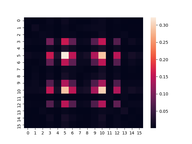
prep_density_matrix = prepare_state(out_params, dev)

We then display the prepared state by plotting a heatmap of the entry-wise absolute value of the density matrix:

seaborn.heatmap(abs(prep_density_matrix))
plt.show()

Numerical Calculations

To verify that we have in fact prepared a good approximation of the thermal state, let’s calculate it numerically by taking the matrix exponential of the Heisenberg Hamiltonian, as was outlined earlier.

def create_target(qubit, beta, ham, graph):

    # Calculates the matrix form of the density matrix, by taking
    # the exponential of the Hamiltonian

    h = ham(qubit, graph)
    y = -1 * float(beta) * h
    new_matrix = scipy.linalg.expm(np.array(y))
    norm = np.trace(new_matrix)
    final_target = (1 / norm) * new_matrix

    return final_target


target_density_matrix = create_target(
    nr_qubits, beta,
    create_hamiltonian_matrix,
    interaction_graph
    )

Finally, we can plot a heatmap of the target density matrix:

seaborn.heatmap(abs(target_density_matrix))
plt.show()

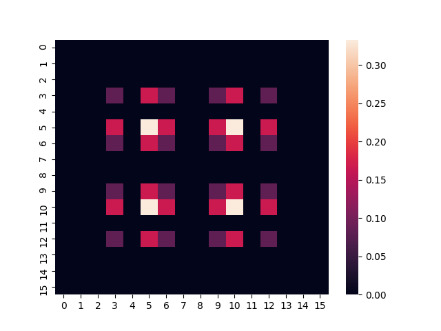
The two images look very similar, which suggests that we have constructed a good approximation of the thermal state! Alternatively, if you prefer a more quantitative measure of similarity, we can calculate the trace distance between the two density matrices, which is defined as

\[T(\rho, \ \sigma) \ = \ \frac{1}{2} \text{Tr} \sqrt{(\rho \ - \ \sigma)^{\dagger} (\rho \ - \ \sigma)},\]

and is a metric on the space of density matrices:

def trace_distance(one, two):

    return 0.5 * np.trace(np.absolute(np.add(one, -1 * two)))


print("Trace Distance: " + str(trace_distance(target_density_matrix, prep_density_matrix)))

Out:

Trace Distance: 0.07226274732179323

The closer to zero, the more similar the two states are. Thus, we have found a close approximation of the thermal state of \(H\) with the VQT!

References

1. Verdon, G., Marks, J., Nanda, S., Leichenauer, S., & Hidary, J. (2019). Quantum Hamiltonian-Based Models and the Variational Quantum Thermalizer Algorithm. arXiv preprint arXiv:1910.02071.

About the author

Jack Ceroni

Jack is currently a second-year undergraduate student at the University of Toronto, pursuing a degree in pure mathematics. Broadly, his interests are related to simulating quantum systems with quantum computers, mathematical abstraction, and philosophy.

demos/tutorial_vqt

 

Download Python script

 

Download Notebook

 

View on GitHub