Quantum natural gradient

Author: Josh Izaac — Posted: 11 October 2019. Last updated: 25 January 2021.

This example demonstrates the quantum natural gradient optimization technique for variational quantum circuits, originally proposed in Stokes et al. (2019).

Background

The most successful class of quantum algorithms for use on near-term noisy quantum hardware is the so-called variational quantum algorithm. As laid out in the Concepts section, in variational quantum algorithms a low-depth parametrized quantum circuit ansatz is chosen, and a problem-specific observable measured. A classical optimization loop is then used to find the set of quantum parameters that minimize a particular measurement expectation value of the quantum device. Examples of such algorithms include the variational quantum eigensolver (VQE), the quantum approximate optimization algorithm (QAOA), and quantum neural networks (QNN).

Most recent demonstrations of variational quantum algorithms have used gradient-free classical optimization methods, such as the Nelder-Mead algorithm. However, the parameter-shift rule (as implemented in PennyLane) allows the user to automatically compute analytic gradients of quantum circuits. This opens up the possibility to train quantum computing hardware using gradient descent—the same method used to train deep learning models. Though one caveat has surfaced with gradient descent — how do we choose the optimal step size for our variational quantum algorithms, to ensure successful and efficient optimization?

The natural gradient

In standard gradient descent, each optimization step is given by

\[\theta_{t+1} = \theta_t -\eta \nabla \mathcal{L}(\theta),\]

where \(\mathcal{L}(\theta)\) is the cost as a function of the parameters \(\theta\), and \(\eta\) is the learning rate or step size. In essence, each optimization step calculates the steepest descent direction around the local value of \(\theta_t\) in the parameter space, and updates \(\theta_t\rightarrow \theta_{t+1}\) by this vector.

The problem with the above approach is that each optimization step is strongly connected to a Euclidean geometry on the parameter space. The parametrization is not unique, and different parametrizations can distort distances within the optimization landscape.

For example, consider the following cost function \(\mathcal{L}\), parametrized using two different coordinate systems, \((\theta_0, \theta_1)\), and \((\phi_0, \phi_1)\):

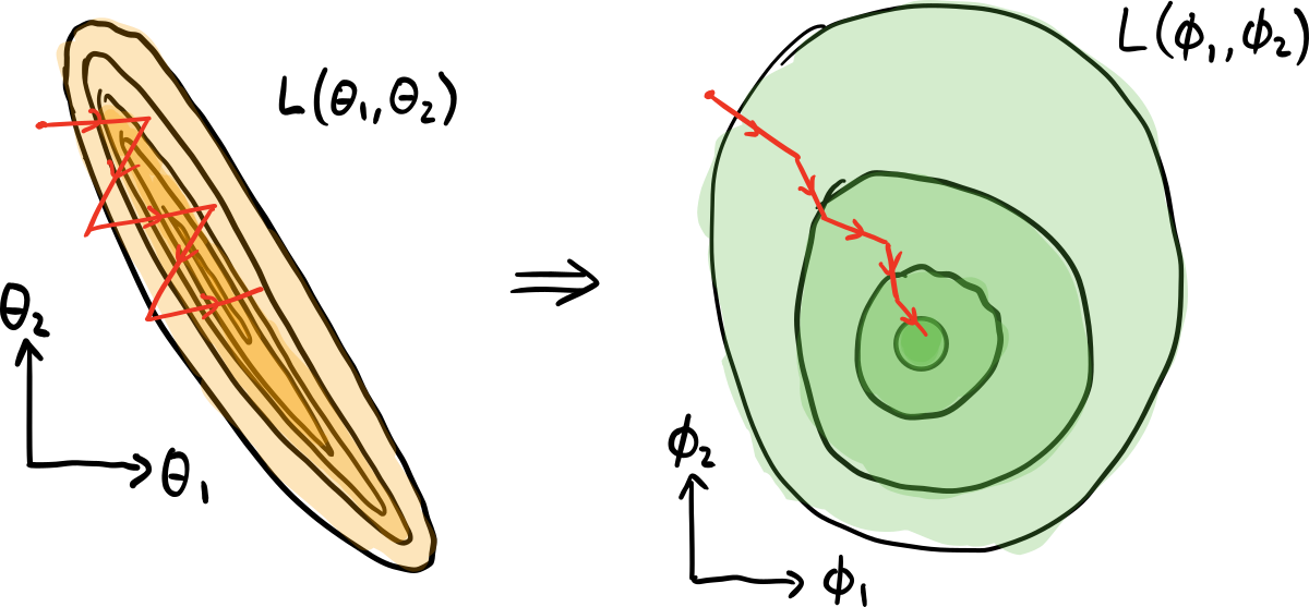
Performing gradient descent in the \((\theta_0, \theta_1)\) parameter space, we are updating each parameter by the same Euclidean distance, and not taking into account the fact that the cost function might vary at a different rate with respect to each parameter.

Instead, if we perform a change of coordinate system (re-parametrization) of the cost function, we might find a parameter space where variations in \(\mathcal{L}\) are similar across different parameters. This is the case with the new parametrization \((\phi_0, \phi_1)\); the cost function is unchanged, but we now have a nicer geometry in which to perform gradient descent, and a more informative stepsize. This leads to faster convergence, and can help avoid optimization becoming stuck in local minima. For a more in-depth explanation, including why the parameter space might not be best represented by a Euclidean space, see Yamamoto (2019).

However, what if we avoid gradient descent in the parameter space altogether? If we instead consider the optimization problem as a probability distribution of possible output values given an input (i.e., maximum likelihood estimation), a better approach is to perform the gradient descent in the distribution space, which is dimensionless and invariant with respect to the parametrization. As a result, each optimization step will always choose the optimum step-size for every parameter, regardless of the parametrization.

In classical neural networks, the above process is known as natural gradient descent, and was first introduced by Amari (1998). The standard gradient descent is modified as follows:

\[\theta_{t+1} = \theta_t - \eta F^{-1}\nabla \mathcal{L}(\theta),\]

where \(F\) is the Fisher information matrix. The Fisher information matrix acts as a metric tensor, transforming the steepest descent in the Euclidean parameter space to the steepest descent in the distribution space.

The quantum analog

In a similar vein, it has been shown that the standard Euclidean geometry is sub-optimal for optimization of quantum variational algorithms (Harrow and Napp, 2019). The space of quantum states instead possesses a unique invariant metric tensor known as the Fubini-Study metric tensor \(g_{ij}\), which can be used to construct a quantum analog to natural gradient descent:

\[\theta_{t+1} = \theta_t - \eta g^{+}(\theta_t)\nabla \mathcal{L}(\theta),\]

where \(g^{+}\) refers to the pseudo-inverse.

Note

It can be shown that the Fubini-Study metric tensor reduces to the Fisher information matrix in the classical limit.

Furthermore, in the limit where \(\eta\rightarrow 0\), the dynamics of the system are equivalent to imaginary-time evolution within the variational subspace, as proposed in McArdle et al. (2018).

Block-diagonal metric tensor

A block-diagonal approximation to the Fubini-Study metric tensor of a variational quantum circuit can be evaluated on quantum hardware.

Consider a variational quantum circuit

\[U(\mathbf{\theta})|\psi_0\rangle = V_L(\theta_L) W_L V_{L-1}(\theta_{L-1}) W_{L-1} \cdots V_{\ell}(\theta_{\ell}) W_{\ell} \cdots V_{0}(\theta_{0}) W_{0} |\psi_0\rangle\]

where

• \(|\psi_0\rangle\) is the initial state,

• \(W_\ell\) are layers of non-parametrized quantum gates,

• \(V_\ell(\theta_\ell)\) are layers of parametrized quantum gates with \(n_\ell\) parameters \(\theta_\ell = \{\theta^{(\ell)}_0, \dots, \theta^{(\ell)}_n\}\).

Further, assume all parametrized gates can be written in the form \(X(\theta^{(\ell)}_{i}) = e^{i\theta^{(\ell)}_{i} K^{(\ell)}_i}\), where \(K^{(\ell)}_i\) is the generator of the parametrized operation.

For each parametric layer \(\ell\) in the variational quantum circuit the \(n_\ell\times n_\ell\) block-diagonal submatrix of the Fubini-Study tensor \(g_{ij}^{(\ell)}\) is calculated by:

\[g_{ij}^{(\ell)} = \langle \psi_{\ell-1} | K_i K_j | \psi_{\ell-1} \rangle - \langle \psi_{\ell-1} | K_i | \psi_{\ell-1}\rangle \langle \psi_{\ell-1} |K_j | \psi_{\ell-1}\rangle\]

where

\[| \psi_{\ell-1}\rangle = V_{\ell-1}(\theta_{\ell-1}) W_{\ell-1} \cdots V_{0}(\theta_{0}) W_{0} |\psi_0\rangle.\]

(that is, \(|\psi_{\ell-1}\rangle\) is the quantum state prior to the application of parameterized layer \(\ell\)), and we have \(K_i \equiv K_i^{(\ell)}\) for brevity.

Let’s consider a small variational quantum circuit example coded in PennyLane:

import pennylane as qml
from pennylane import numpy as np

dev = qml.device("default.qubit", wires=3)


@qml.qnode(dev, interface="autograd")
def circuit(params):
    # |psi_0>: state preparation
    qml.RY(np.pi / 4, wires=0)
    qml.RY(np.pi / 3, wires=1)
    qml.RY(np.pi / 7, wires=2)

    # V0(theta0, theta1): Parametrized layer 0
    qml.RZ(params[0], wires=0)
    qml.RZ(params[1], wires=1)

    # W1: non-parametrized gates
    qml.CNOT(wires=[0, 1])
    qml.CNOT(wires=[1, 2])

    # V_1(theta2, theta3): Parametrized layer 1
    qml.RY(params[2], wires=1)
    qml.RX(params[3], wires=2)

    # W2: non-parametrized gates
    qml.CNOT(wires=[0, 1])
    qml.CNOT(wires=[1, 2])

    return qml.expval(qml.PauliY(0))


params = np.array([0.432, -0.123, 0.543, 0.233])

The above circuit consists of 4 parameters, with two distinct parametrized layers of 2 parameters each.

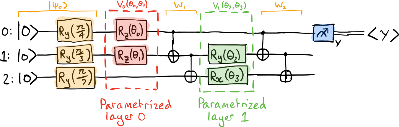
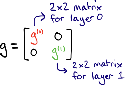
(Note that in this example, the first non-parametrized layer \(W_0\) is simply the identity.) Since there are two layers, each with two parameters, the block-diagonal approximation consists of two \(2\times 2\) matrices, \(g^{(0)}\) and \(g^{(1)}\).

To compute the first block-diagonal \(g^{(0)}\), we create subcircuits consisting of all gates prior to the layer, and observables corresponding to the generators of the gates in the layer:

g0 = np.zeros([2, 2])


def layer0_subcircuit(params):
    """This function contains all gates that
    precede parametrized layer 0"""
    qml.RY(np.pi / 4, wires=0)
    qml.RY(np.pi / 3, wires=1)
    qml.RY(np.pi / 7, wires=2)

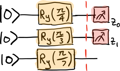
We then post-process the measurement results in order to determine \(g^{(0)}\), as follows.

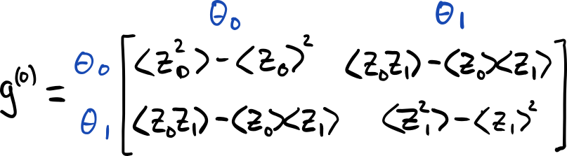
We can see that the diagonal terms are simply given by the variance:

@qml.qnode(dev, interface="autograd")
def layer0_diag(params):
    layer0_subcircuit(params)
    return qml.var(qml.PauliZ(0)), qml.var(qml.PauliZ(1))


# calculate the diagonal terms
varK0, varK1 = layer0_diag(params)
g0[0, 0] = varK0 / 4
g0[1, 1] = varK1 / 4

The following two subcircuits are then used to calculate the off-diagonal covariance terms of \(g^{(0)}\):

@qml.qnode(dev, interface="autograd")
def layer0_off_diag_single(params):
    layer0_subcircuit(params)
    return qml.expval(qml.PauliZ(0)), qml.expval(qml.PauliZ(1))


@qml.qnode(dev, interface="autograd")
def layer0_off_diag_double(params):
    layer0_subcircuit(params)
    ZZ = np.kron(np.diag([1, -1]), np.diag([1, -1]))
    return qml.expval(qml.Hermitian(ZZ, wires=[0, 1]))


# calculate the off-diagonal terms
exK0, exK1 = layer0_off_diag_single(params)
exK0K1 = layer0_off_diag_double(params)

g0[0, 1] = (exK0K1 - exK0 * exK1) / 4
g0[1, 0] = (exK0K1 - exK0 * exK1) / 4

Note that, by definition, the block-diagonal matrices must be real and symmetric.

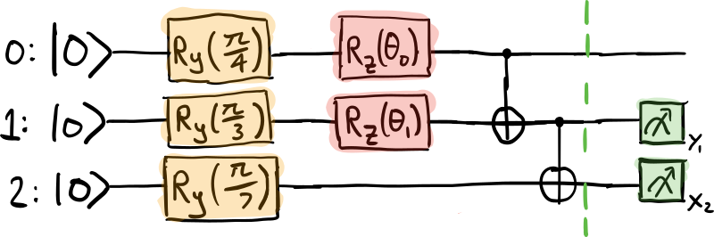
We can repeat the above process to compute \(g^{(1)}\). The subcircuit required is given by

g1 = np.zeros([2, 2])


def layer1_subcircuit(params):
    """This function contains all gates that
    precede parametrized layer 1"""
    # |psi_0>: state preparation
    qml.RY(np.pi / 4, wires=0)
    qml.RY(np.pi / 3, wires=1)
    qml.RY(np.pi / 7, wires=2)

    # V0(theta0, theta1): Parametrized layer 0
    qml.RZ(params[0], wires=0)
    qml.RZ(params[1], wires=1)

    # W1: non-parametrized gates
    qml.CNOT(wires=[0, 1])
    qml.CNOT(wires=[1, 2])

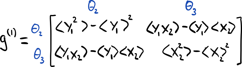
Using this subcircuit, we can now generate the submatrix \(g^{(1)}\).

@qml.qnode(dev, interface="autograd")
def layer1_diag(params):
    layer1_subcircuit(params)
    return qml.var(qml.PauliY(1)), qml.var(qml.PauliX(2))

As previously, the diagonal terms are simply given by the variance,

varK0, varK1 = layer1_diag(params)
g1[0, 0] = varK0 / 4
g1[1, 1] = varK1 / 4

while the off-diagonal terms require covariance between the two observables to be computed.

@qml.qnode(dev, interface="autograd")
def layer1_off_diag_single(params):
    layer1_subcircuit(params)
    return qml.expval(qml.PauliY(1)), qml.expval(qml.PauliX(2))


@qml.qnode(dev, interface="autograd")
def layer1_off_diag_double(params):
    layer1_subcircuit(params)
    X = np.array([[0, 1], [1, 0]])
    Y = np.array([[0, -1j], [1j, 0]])
    YX = np.kron(Y, X)
    return qml.expval(qml.Hermitian(YX, wires=[1, 2]))


# calculate the off-diagonal terms
exK0, exK1 = layer1_off_diag_single(params)
exK0K1 = layer1_off_diag_double(params)

g1[0, 1] = (exK0K1 - exK0 * exK1) / 4
g1[1, 0] = g1[0, 1]

Putting this altogether, the block-diagonal approximation to the Fubini-Study metric tensor for this variational quantum circuit is

from scipy.linalg import block_diag

g = block_diag(g0, g1)
print(np.round(g, 8))

Out:

[[ 0.125      -0.          0.          0.        ]
 [-0.          0.1875      0.          0.        ]
 [ 0.          0.          0.24973433 -0.01524701]
 [ 0.          0.         -0.01524701  0.20293623]]

PennyLane contains a built-in function for computing the Fubini-Study metric tensor, metric_tensor(), which we can use to verify this result:

print(np.round(qml.metric_tensor(circuit, approx="block-diag")(params), 8))

Out:

[[ 0.125       0.          0.          0.        ]
 [ 0.          0.1875      0.          0.        ]
 [ 0.          0.          0.24973433 -0.01524701]
 [ 0.          0.         -0.01524701  0.20293623]]

As opposed to our manual computation, which required 6 different quantum evaluations, the PennyLane Fubini-Study metric tensor implementation requires only 2 quantum evaluations, one per layer. This is done by automatically detecting the layer structure, and noting that every observable that must be measured commutes, allowing for simultaneous measurement.

Therefore, by combining the quantum natural gradient optimizer with the analytic parameter-shift rule to optimize a variational circuit with \(d\) parameters and \(L\) parametrized layers, a total of \(2d+L\) quantum evaluations are required per optimization step.

Note that the metric_tensor() function also supports computing the diagonal approximation to the metric tensor:

print(qml.metric_tensor(circuit, approx='diag')(params))

Out:

[[0.125      0.         0.         0.        ]
 [0.         0.1875     0.         0.        ]
 [0.         0.         0.24973433 0.        ]
 [0.         0.         0.         0.20293623]]

Furthermore, the returned metric tensor is full differentiable; include it in your cost function, and train or optimize its value!

Quantum natural gradient optimization

PennyLane provides an implementation of the quantum natural gradient optimizer, QNGOptimizer. Let’s compare the optimization convergence of the QNG Optimizer and the GradientDescentOptimizer for the simple variational circuit above.

steps = 200
init_params = np.array([0.432, -0.123, 0.543, 0.233], requires_grad=True)

Performing vanilla gradient descent:

gd_cost = []
opt = qml.GradientDescentOptimizer(0.01)

theta = init_params
for _ in range(steps):
    theta = opt.step(circuit, theta)
    gd_cost.append(circuit(theta))

Performing quantum natural gradient descent:

qng_cost = []
opt = qml.QNGOptimizer(0.01)

theta = init_params
for _ in range(steps):
    theta = opt.step(circuit, theta)
    qng_cost.append(circuit(theta))

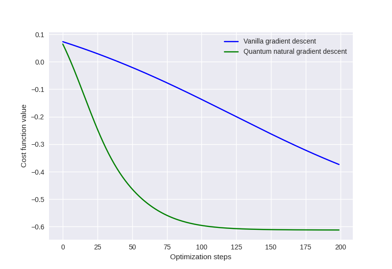
Plotting the cost vs optimization step for both optimization strategies:

from matplotlib import pyplot as plt

plt.style.use("seaborn")
plt.plot(gd_cost, "b", label="Vanilla gradient descent")
plt.plot(qng_cost, "g", label="Quantum natural gradient descent")

plt.ylabel("Cost function value")
plt.xlabel("Optimization steps")
plt.legend()
plt.show()

References

1. Shun-Ichi Amari. “Natural gradient works efficiently in learning.” Neural computation 10.2, 251-276, 1998.

2. James Stokes, Josh Izaac, Nathan Killoran, Giuseppe Carleo. “Quantum Natural Gradient.” arXiv:1909.02108, 2019.

3. Aram Harrow and John Napp. “Low-depth gradient measurements can improve convergence in variational hybrid quantum-classical algorithms.” arXiv:1901.05374, 2019.

4. Naoki Yamamoto. “On the natural gradient for variational quantum eigensolver.” arXiv:1909.05074, 2019.

About the author

Josh Izaac

Josh is a theoretical physicist, software tinkerer, and occasional baker. At Xanadu, he contributes to the development and growth of Xanadu’s open-source quantum software products.

demos/tutorial_quantum_natural_gradient

 

Download Python script

 

Download Notebook

 

View on GitHub