Accelerating VQEs with quantum natural gradient

Authors: Maggie Li, Lana Bozanic, Sukin Sim — Posted: 06 November 2020. Last updated: 08 April 2021.

This tutorial showcases how one can apply quantum natural gradients (QNG) 1 2 to accelerate the optimization step of the Variational Quantum Eigensolver (VQE) algorithm 3. We will implement two small examples: estimating the ground state energy of a single-qubit VQE problem, which we can visualize using the Bloch sphere, and the hydrogen molecule.

Before going through this tutorial, we recommend that readers refer to the QNG tutorial and VQE tutorial for overviews of quantum natural gradient and the variational quantum eigensolver algorithm, respectively. Let’s get started!

Single-qubit VQE example

The first step is to import the required libraries and packages:

import matplotlib.pyplot as plt
from pennylane import numpy as np
import pennylane as qml

For this simple example, we consider the following single-qubit Hamiltonian: \(\sigma_x + \sigma_z\).

We define the device:

dev = qml.device("default.qubit", wires=1)

For the variational ansatz, we use two single-qubit rotations, which the user may recognize from a previous tutorial on qubit rotations.

def circuit(params, wires=0):
    qml.RX(params[0], wires=wires)
    qml.RY(params[1], wires=wires)

We then define our cost function which supports the computation of block-diagonal or diagonal approximations to the Fubini-Study metric tensor 1. This tensor is a crucial component for optimizing with quantum natural gradients.

coeffs = [1, 1]
obs = [qml.PauliX(0), qml.PauliZ(0)]

H = qml.Hamiltonian(coeffs, obs)

@qml.qnode(dev, interface="autograd")
def cost_fn(params):
    circuit(params)
    return qml.expval(H)

To analyze the performance of quantum natural gradient on VQE calculations, we set up and execute optimizations using the GradientDescentOptimizer (which does not utilize quantum gradients) and the QNGOptimizer that uses the block-diagonal approximation to the metric tensor.

To perform a fair comparison, we fix the initial parameters for the two optimizers.

init_params = np.array([3.97507603, 3.00854038], requires_grad=True)

We will carry out each optimization over a maximum of 500 steps. As was done in the VQE tutorial, we aim to reach a convergence tolerance of around \(10^{-6}\). We use a step size of 0.01.

max_iterations = 500
conv_tol = 1e-06
step_size = 0.01

First, we carry out the VQE optimization using the standard gradient descent method.

opt = qml.GradientDescentOptimizer(stepsize=step_size)

params = init_params

gd_param_history = [params]
gd_cost_history = []

for n in range(max_iterations):

    # Take step
    params, prev_energy = opt.step_and_cost(cost_fn, params)
    gd_param_history.append(params)
    gd_cost_history.append(prev_energy)

    energy = cost_fn(params)

    # Calculate difference between new and old energies
    conv = np.abs(energy - prev_energy)

    if n % 20 == 0:
        print(
            "Iteration = {:},  Energy = {:.8f} Ha,  Convergence parameter = {"
            ":.8f} Ha".format(n, energy, conv)
        )

    if conv <= conv_tol:
        break

print()
print("Final value of the energy = {:.8f} Ha".format(energy))
print("Number of iterations = ", n)

Out:

Iteration = 0,  Energy = 0.56743624 Ha,  Convergence parameter = 0.00973536 Ha
Iteration = 20,  Energy = 0.38709233 Ha,  Convergence parameter = 0.00821261 Ha
Iteration = 40,  Energy = 0.24420954 Ha,  Convergence parameter = 0.00616395 Ha
Iteration = 60,  Energy = 0.14079686 Ha,  Convergence parameter = 0.00435028 Ha
Iteration = 80,  Energy = 0.06758408 Ha,  Convergence parameter = 0.00314443 Ha
Iteration = 100,  Energy = 0.01128048 Ha,  Convergence parameter = 0.00262544 Ha
Iteration = 120,  Energy = -0.04175219 Ha,  Convergence parameter = 0.00278160 Ha
Iteration = 140,  Energy = -0.10499504 Ha,  Convergence parameter = 0.00361450 Ha
Iteration = 160,  Energy = -0.19195848 Ha,  Convergence parameter = 0.00511056 Ha
Iteration = 180,  Energy = -0.31444953 Ha,  Convergence parameter = 0.00708743 Ha
Iteration = 200,  Energy = -0.47706980 Ha,  Convergence parameter = 0.00900220 Ha
Iteration = 220,  Energy = -0.66993027 Ha,  Convergence parameter = 0.01001574 Ha
Iteration = 240,  Energy = -0.86789981 Ha,  Convergence parameter = 0.00955105 Ha
Iteration = 260,  Energy = -1.04241317 Ha,  Convergence parameter = 0.00783834 Ha
Iteration = 280,  Energy = -1.17653061 Ha,  Convergence parameter = 0.00567546 Ha
Iteration = 300,  Energy = -1.26906291 Ha,  Convergence parameter = 0.00374812 Ha
Iteration = 320,  Energy = -1.32823089 Ha,  Convergence parameter = 0.00232769 Ha
Iteration = 340,  Energy = -1.36424033 Ha,  Convergence parameter = 0.00139097 Ha
Iteration = 360,  Energy = -1.38549883 Ha,  Convergence parameter = 0.00081221 Ha
Iteration = 380,  Energy = -1.39782393 Ha,  Convergence parameter = 0.00046788 Ha
Iteration = 400,  Energy = -1.40489478 Ha,  Convergence parameter = 0.00026743 Ha
Iteration = 420,  Energy = -1.40892679 Ha,  Convergence parameter = 0.00015217 Ha
Iteration = 440,  Energy = -1.41121801 Ha,  Convergence parameter = 0.00008637 Ha
Iteration = 460,  Energy = -1.41251745 Ha,  Convergence parameter = 0.00004895 Ha
Iteration = 480,  Energy = -1.41325360 Ha,  Convergence parameter = 0.00002772 Ha

Final value of the energy = -1.41365468 Ha
Number of iterations =  499

We then repeat the process for the optimizer employing quantum natural gradients:

opt = qml.QNGOptimizer(stepsize=step_size, approx="block-diag")

params = init_params

qngd_param_history = [params]
qngd_cost_history = []

for n in range(max_iterations):

    # Take step
    params, prev_energy = opt.step_and_cost(cost_fn, params)
    qngd_param_history.append(params)
    qngd_cost_history.append(prev_energy)

    # Compute energy
    energy = cost_fn(params)

    # Calculate difference between new and old energies
    conv = np.abs(energy - prev_energy)

    if n % 20 == 0:
        print(
            "Iteration = {:},  Energy = {:.8f} Ha,  Convergence parameter = {"
            ":.8f} Ha".format(n, energy, conv)
        )

    if conv <= conv_tol:
        break

print()
print("Final value of the energy = {:.8f} Ha".format(energy))
print("Number of iterations = ", n)

Out:

Iteration = 0,  Energy = 0.51052556 Ha,  Convergence parameter = 0.06664604 Ha
Iteration = 20,  Energy = -0.90729965 Ha,  Convergence parameter = 0.05006082 Ha
Iteration = 40,  Energy = -1.35504644 Ha,  Convergence parameter = 0.00713113 Ha
Iteration = 60,  Energy = -1.40833787 Ha,  Convergence parameter = 0.00072399 Ha
Iteration = 80,  Energy = -1.41364035 Ha,  Convergence parameter = 0.00007078 Ha
Iteration = 100,  Energy = -1.41415774 Ha,  Convergence parameter = 0.00000689 Ha

Final value of the energy = -1.41420585 Ha
Number of iterations =  117

Visualizing the results

For single-qubit examples, we can visualize the optimization process in several ways.

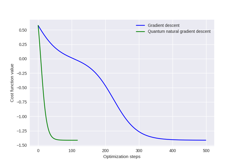
For example, we can track the energy history:

plt.style.use("seaborn")
plt.plot(gd_cost_history, "b", label="Gradient descent")
plt.plot(qngd_cost_history, "g", label="Quantum natural gradient descent")

plt.ylabel("Cost function value")
plt.xlabel("Optimization steps")
plt.legend()
plt.show()

Or we can visualize the optimization path in the parameter space using a contour plot. Energies at different grid points have been pre-computed, and they can be downloaded by clicking here.

# Discretize the parameter space
theta0 = np.linspace(0.0, 2.0 * np.pi, 100)
theta1 = np.linspace(0.0, 2.0 * np.pi, 100)

# Load energy value at each point in parameter space
parameter_landscape = np.load("vqe_qng/param_landscape.npy")

# Plot energy landscape
fig, axes = plt.subplots(figsize=(6, 6))
cmap = plt.cm.get_cmap("coolwarm")
contour_plot = plt.contourf(theta0, theta1, parameter_landscape, cmap=cmap)
plt.xlabel(r"$\theta_0$")
plt.ylabel(r"$\theta_1$")

# Plot optimization path for gradient descent. Plot every 10th point.
gd_color = "g"
plt.plot(
    np.array(gd_param_history)[::10, 0],
    np.array(gd_param_history)[::10, 1],
    ".",
    color=gd_color,
    linewidth=1,
    label="Gradient descent",
)
plt.plot(
    np.array(gd_param_history)[:, 0],
    np.array(gd_param_history)[:, 1],
    "-",
    color=gd_color,
    linewidth=1,
)

# Plot optimization path for quantum natural gradient descent. Plot every 10th point.
qngd_color = "k"
plt.plot(
    np.array(qngd_param_history)[::10, 0],
    np.array(qngd_param_history)[::10, 1],
    ".",
    color=qngd_color,
    linewidth=1,
    label="Quantum natural gradient descent",
)
plt.plot(
    np.array(qngd_param_history)[:, 0],
    np.array(qngd_param_history)[:, 1],
    "-",
    color=qngd_color,
    linewidth=1,
)

plt.legend()
plt.show()

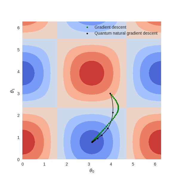
Here, the blue regions indicate states with lower energies, and the red regions indicate states with higher energies. We can see that the QNGOptimizer takes a more direct route to the minimum in larger strides compared to the path taken by the GradientDescentOptimizer.

Lastly, we can visualize the same optimization paths on the Bloch sphere using routines from QuTiP. The result should look like the following:

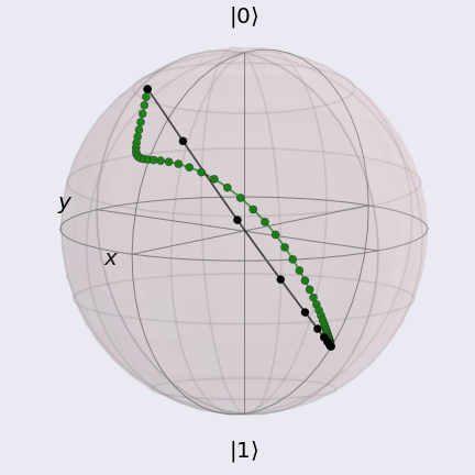
where again the black markers and line indicate the path taken by the QNGOptimizer, and the green markers and line indicate the path taken by the GradientDescentOptimizer. Using this visualization method, we can clearly see how the path using the QNGOptimizer tightly “hugs” the curvature of the Bloch sphere and takes the shorter path.

Now, we will move onto a more interesting example: estimating the ground state energy of molecular hydrogen.

Hydrogen VQE Example

To construct our system Hamiltonian, we first read the molecular geometry from the external file h2.xyz using the read_structure() function (see more details in the Building molecular Hamiltonians tutorial). The molecular Hamiltonian is then built using the molecular_hamiltonian() function.

geo_file = "h2.xyz"

symbols, coordinates = qml.qchem.read_structure(geo_file)
hamiltonian, qubits = qml.qchem.molecular_hamiltonian(symbols, coordinates)

print("Number of qubits = ", qubits)

Out:

Number of qubits =  4

For our ansatz, we use the circuit from the VQE tutorial but expand out the arbitrary single-qubit rotations to elementary gates (RZ-RY-RZ).

dev = qml.device("default.qubit", wires=qubits)
hf_state = np.array([1, 1, 0, 0], requires_grad=False)

def ansatz(params, wires=[0, 1, 2, 3]):
    qml.BasisState(hf_state, wires=wires)
    for i in wires:
        qml.RZ(params[3 * i], wires=i)
        qml.RY(params[3 * i + 1], wires=i)
        qml.RZ(params[3 * i + 2], wires=i)
    qml.CNOT(wires=[2, 3])
    qml.CNOT(wires=[2, 0])
    qml.CNOT(wires=[3, 1])

Note that the qubit register has been initialized to \(|1100\rangle\), which encodes for the Hartree-Fock state of the hydrogen molecule described in the minimal basis. Again, we define the cost function to be the following QNode that measures expval(H):

@qml.qnode(dev, interface="autograd")
def cost(params):
    ansatz(params)
    return qml.expval(hamiltonian)

For this problem, we can compute the exact value of the ground state energy via exact diagonalization. We provide the value below.

exact_value = -1.136189454088

We now set up our optimizations runs.

np.random.seed(0)
init_params = np.random.uniform(low=0, high=2 * np.pi, size=12, requires_grad=True)
max_iterations = 500
step_size = 0.5
conv_tol = 1e-06

As was done with our previous VQE example, we run the standard gradient descent optimizer.

opt = qml.GradientDescentOptimizer(step_size)

params = init_params

gd_cost = []

for n in range(max_iterations):
    params, prev_energy = opt.step_and_cost(cost, params)
    gd_cost.append(prev_energy)

    energy = cost(params)
    conv = np.abs(energy - prev_energy)

    if n % 20 == 0:
        print(
            "Iteration = {:},  Energy = {:.8f} Ha".format(n, energy)
        )

    if conv <= conv_tol:
        break


print()
print("Final convergence parameter = {:.8f} Ha".format(conv))
print("Number of iterations = ", n)
print("Final value of the ground-state energy = {:.8f} Ha".format(energy))
print(
    "Accuracy with respect to the FCI energy: {:.8f} Ha ({:.8f} kcal/mol)".format(
        np.abs(energy - exact_value), np.abs(energy - exact_value) * 627.503
    )
)
print()
print("Final circuit parameters = \n", params)

Out:

Iteration = 0,  Energy = -0.09424333 Ha
Iteration = 20,  Energy = -0.55156841 Ha
Iteration = 40,  Energy = -1.12731586 Ha
Iteration = 60,  Energy = -1.13583263 Ha
Iteration = 80,  Energy = -1.13602366 Ha
Iteration = 100,  Energy = -1.13611095 Ha
Iteration = 120,  Energy = -1.13615238 Ha

Final convergence parameter = 0.00000097 Ha
Number of iterations =  130
Final value of the ground-state energy = -1.13616398 Ha
Accuracy with respect to the FCI energy: 0.00002547 Ha (0.01598208 kcal/mol)

Final circuit parameters =
 [3.44829694e+00 6.28318531e+00 3.78727399e+00 3.42360201e+00
 5.09234599e-08 4.05827240e+00 2.74944154e+00 6.07360302e+00
 6.24620659e+00 2.40923412e+00 6.28318531e+00 3.32314479e+00]

Next, we run the optimizer employing quantum natural gradients. We also need to make the Hamiltonian coefficients non-differentiable by setting requires_grad=False.

hamiltonian = qml.Hamiltonian(np.array(hamiltonian.coeffs, requires_grad=False), hamiltonian.ops)

opt = qml.QNGOptimizer(step_size, lam=0.001, approx="block-diag")

params = init_params
prev_energy = cost(params)
qngd_cost = []

for n in range(max_iterations):
    params, prev_energy = opt.step_and_cost(cost, params)
    qngd_cost.append(prev_energy)

    energy = cost(params)
    conv = np.abs(energy - prev_energy)

    if n % 4 == 0:
        print(
            "Iteration = {:},  Energy = {:.8f} Ha".format(n, energy)
        )

    if conv <= conv_tol:
        break


print("\nFinal convergence parameter = {:.8f} Ha".format(conv))
print("Number of iterations = ", n)
print("Final value of the ground-state energy = {:.8f} Ha".format(energy))
print(
    "Accuracy with respect to the FCI energy: {:.8f} Ha ({:.8f} kcal/mol)".format(
        np.abs(energy - exact_value), np.abs(energy - exact_value) * 627.503
    )
)
print()
print("Final circuit parameters = \n", params)

Out:

Iteration = 0,  Energy = -0.32164519 Ha
Iteration = 4,  Energy = -0.46875033 Ha
Iteration = 8,  Energy = -0.85091050 Ha
Iteration = 12,  Energy = -1.13575339 Ha
Iteration = 16,  Energy = -1.13618916 Ha

Final convergence parameter = 0.00000022 Ha
Number of iterations =  17
Final value of the ground-state energy = -1.13618938 Ha
Accuracy with respect to the FCI energy: 0.00000008 Ha (0.00004847 kcal/mol)

Final circuit parameters =
 [3.44829694e+00 6.28318510e+00 3.78727399e+00 3.42360201e+00
 4.03252276e-04 4.05827240e+00 2.74944154e+00 6.07375181e+00
 6.28402001e+00 2.40923412e+00 6.28318525e+00 3.32314479e+00]

Visualizing the results

To evaluate the performance of our two optimizers, we can compare: (a) the number of steps it takes to reach our ground state estimate and (b) the quality of our ground state estimate by comparing the final optimization energy to the exact value.

plt.style.use("seaborn")
plt.plot(np.array(gd_cost) - exact_value, "g", label="Gradient descent")
plt.plot(np.array(qngd_cost) - exact_value, "k", label="Quantum natural gradient descent")
plt.yscale("log")
plt.ylabel("Energy difference")
plt.xlabel("Step")
plt.legend()
plt.show()

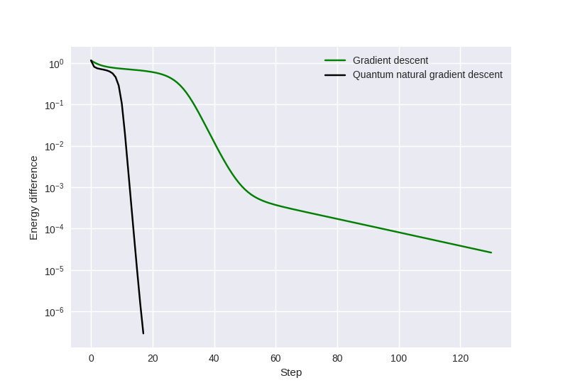
We see that by employing quantum natural gradients, it takes fewer steps to reach a ground state estimate and the optimized energy achieved by the optimizer is lower than that obtained using vanilla gradient descent.

Robustness in parameter initialization

While results above show a more rapid convergence for quantum natural gradients, what if we were just lucky, i.e., we started at a “good” point in parameter space? How do we know this will be the case with high probability regardless of the parameter initialization?

Using the same system Hamiltonian, ansatz, and device, we tested the robustness of the QNGOptimizer by running 10 independent trials with random parameter initializations. For this numerical test, our optimizer does not terminate based on energy improvement; we fix the number of iterations to 200. We show the result of this test below (after pre-computing), where we plot the mean and standard deviation of the energies over optimization steps for quantum natural gradient and standard gradient descent.

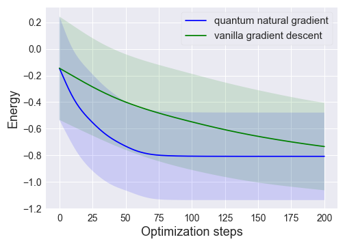
We observe that quantum natural gradient on average converges faster for this system.

Note

While using QNG may help accelerate the VQE algorithm in terms of optimization steps, each QNG step is more costly than its vanilla gradient descent counterpart due to a greater number of calls to the quantum computer that are needed to compute the Fubini-Study metric tensor.

While further benchmark studies are needed to better understand the advantages of quantum natural gradient, preliminary studies such as this tutorial show the potentials of the method. 🎉

References

1(1,2)

Stokes, James, et al., “Quantum Natural Gradient”. arXiv preprint arXiv:1909.02108 (2019).

2

Yamamoto, Naoki, “On the natural gradient for variational quantum eigensolver”. arXiv preprint arXiv:1909.05074 (2019).

3

Alberto Peruzzo, Jarrod McClean et al., “A variational eigenvalue solver on a photonic quantum processor”. Nature Communications 5, 4213 (2014).

About the authors

Maggie Li

Maggie is a student interested in how quantum computing and information theory can be applied to and inform our understanding of biology.

Lana Bozanic

Lana is a Mathematical Physics undergraduate at the University of Waterloo. She has spent time pursuing her research interests in quantum optics at the Institute for Quantum Computing (IQC) & the University of Ottawa, as well as particle physics at the University of Toronto.

Sukin Sim

Sukin (Dylan) completed their PhD in Chemical Physics at Harvard University and currently works as a quantum research scientist. Their research interests include the development of algorithms and circuit compilation schemes for fault-tolerant quantum computers.

demos/tutorial_vqe_qng

 

Download Python script

 

Download Notebook

 

View on GitHub