Quantum circuit structure learning

Author: Angus Lowe — Posted: 16 October 2019. Last updated: 20 January 2021.

This example shows how to learn a good selection of rotation gates so as to minimize a cost function using the Rotoselect algorithm of Ostaszewski et al. (2019). We apply this algorithm to minimize a Hamiltonian for a variational quantum eigensolver (VQE) problem, and improve upon an initial circuit structure ansatz.

Note

The Rotoselect and Rotosolve algorithms are directly implemented and available in PennyLane via the optimizers RotoselectOptimizer and RotosolveOptimizer, respectively.

Background

In quantum machine learning and optimization problems, one wishes to minimize a cost function with respect to some parameters in the circuit. It is desirable to keep the circuit as shallow as possible to reduce the effects of noise, but an arbitrary choice of gates is generally suboptimal for performing the optimization. Therefore, it would be useful to employ an algorithm which learns a good circuit structure at fixed depth to minimize the cost function.

Furthermore, PennyLane’s optimizers perform automatic differentiation of quantum nodes by evaluating phase-shifted expectation values using the quantum circuit itself. The output of these calculations, the gradient, is used in optimization methods to minimize the cost function. However, there exists a technique to discover the optimal parameters of a quantum circuit through phase-shifted evaluations, without the need for calculating the gradient as an intermediate step (i.e., a gradient-free optimization). It could be desirable, in some cases, to take advantage of this.

The Rotoselect algorithm addresses the above two points: it allows one to jump directly to the optimal value for a single parameter with respect to fixed values for the other parameters, skipping gradient descent, and tries various rotation gates along the way. The algorithm works by updating the parameters \(\boldsymbol{\theta}=\theta_1,\dots,\theta_D\) and gate choices \(\boldsymbol{R}=R_1,\dots,R_D\) one at a time according to a closed-form expression for the optimal value of the \(d^{\text{th}}\) parameter \(\theta^{*}_d\) when the other parameters and gate choices are fixed:

\[\begin{split}\theta^{*}_d &= \underset{\theta_d}{\text{argmin}} \langle H \rangle_{\theta_d} \\ &= -\frac{\pi}{2} - \text{arctan}\left(\frac{2\langle H \rangle_{\theta_d = 0} - \langle H \rangle_{\theta_d=\pi/2} - \langle H \rangle_{\theta_d=-\pi/2}}{\langle H \rangle_{\theta_d=\pi/2} - \langle H \rangle_{\theta_d=-\pi/2}}\right)\end{split}\]

The calculation makes use of 3 separate evaluations of the expectation value \(\langle H \rangle_{\theta_d}\) using the quantum circuit. Although \(\langle H \rangle\) is really a function of all parameters and gate choices (\(\boldsymbol{\theta}\), \(\boldsymbol{R}\)), we are fixing every parameter and gate choice apart from \(\theta_d\) in this expression so we write it as \(\langle H \rangle = \langle H \rangle_{\theta_d}\). For each parameter in the quantum circuit, the algorithm proceeds by evaluating \(\theta^{*}_d\) for each choice of gate \(R_d \in \{R_x,R_y,R_z\}\) and selecting the gate which yields the minimum value of \(\langle H \rangle\).

Thus, one might expect the number of circuit evaluations required to be 9 for each parameter (3 for each gate choice). However, since all 3 rotation gates yield identity when \(\theta_d=0\),

\[R_x(0) = R_y(0) = R_z(0) = 1,\]

the value of \(\langle H \rangle_{\theta_d=0}\) in the expression for \(\theta_d^{*}\) above is the same for each of the gate choices, and this 3-fold degeneracy reduces the number of evaluations required to 7.

One cycle of the Rotoselect algorithm involves iterating through every parameter and performing the calculation above. This cycle is repeated for a fixed number of steps or until convergence. In this way, one could learn both the optimal parameters and gate choices for the task of minimizing a given cost function. Next, we present an example of this algorithm applied to a VQE Hamiltonian.

Example VQE Problem

We focus on a 2-qubit VQE circuit for simplicity. Here, the Hamiltonian is

\[H = 0.5Y_2 + 0.8Z_1 - 0.2X_1\]

where the subscript denotes the qubit upon which the Pauli operator acts. The expectation value of this quantity acts as the cost function for our optimization.

Rotosolve

As a precursor to implementing Rotoselect we can analyze a version of the algorithm which does not optimize the choice of gates and only optimizes the parameters for a given circuit ansatz, called Rotosolve. Later, we will build on this example to implement Rotoselect and vary the circuit structure.

Imports

To get started, we import PennyLane and the PennyLane-wrapped version of NumPy. We also create a 2-qubit device using the default.qubit plugin and set the analytic keyword to True in order to obtain exact values for any expectation values calculated. In contrast to real devices, simulators have the capability of doing these calculations without sampling.

import pennylane as qml
from pennylane import numpy as np

n_wires = 2

dev = qml.device("default.qubit", shots=1000, wires=2)

Creating a fixed quantum circuit

Next, we set up a circuit with a fixed ansatz structure—which will later be subject to change—and encode the Hamiltonian into a cost function. The structure is shown in the figure above.

def ansatz(params):
    qml.RX(params[0], wires=0)
    qml.RY(params[1], wires=1)
    qml.CNOT(wires=[0, 1])


@qml.qnode(dev)
def circuit(params):
    ansatz(params)
    return qml.expval(qml.PauliZ(0)), qml.expval(qml.PauliY(1))


@qml.qnode(dev)
def circuit2(params):
    ansatz(params)
    return qml.expval(qml.PauliX(0))


def cost(params):
    Z_1, Y_2 = circuit(params)
    X_1 = circuit2(params)
    return 0.5 * Y_2 + 0.8 * Z_1 - 0.2 * X_1

Helper methods for the algorithm

We define methods to evaluate the expression in the previous section. These will serve as the basis for our optimization algorithm.

# calculation as described above
def opt_theta(d, params, cost):
    params[d] = 0.0
    M_0 = cost(params)
    params[d] = np.pi / 2.0
    M_0_plus = cost(params)
    params[d] = -np.pi / 2.0
    M_0_minus = cost(params)
    a = np.arctan2(
        2.0 * M_0 - M_0_plus - M_0_minus, M_0_plus - M_0_minus
    )  # returns value in (-pi,pi]
    params[d] = -np.pi / 2.0 - a
    # restrict output to lie in (-pi,pi], a convention
    # consistent with the Rotosolve paper
    if params[d] <= -np.pi:
        params[d] += 2 * np.pi


# one cycle of rotosolve
def rotosolve_cycle(cost, params):
    for d in range(len(params)):
        opt_theta(d, params, cost)
    return params

Optimization and comparison with gradient descent

We set up some initial parameters for the \(R_x\) and \(R_y\) gates in the ansatz circuit structure and perform an optimization using the Rotosolve algorithm.

init_params = np.array([0.3, 0.25], requires_grad=True)
params_rsol = init_params.copy()
n_steps = 30

costs_rotosolve = []

for i in range(n_steps):
    costs_rotosolve.append(cost(params_rsol))
    params_rsol = rotosolve_cycle(cost, params_rsol)

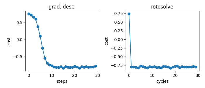
We then compare the results of Rotosolve to an optimization performed with gradient descent and plot the cost functions at each step (or cycle in the case of Rotosolve). This comparison is fair since the number of circuit evaluations involved in a cycle of Rotosolve is similar to those required to calculate the gradient of the circuit and step in this direction. Evidently, the Rotosolve algorithm converges on the minimum after the first cycle for this simple circuit.

params_gd = init_params.copy()
opt = qml.GradientDescentOptimizer(stepsize=0.5)
costs_gd = []
for i in range(n_steps):
    costs_gd.append(cost(params_gd))
    params_gd = opt.step(cost, params_gd)


# plot cost function optimization using the 2 techniques
import matplotlib.pyplot as plt

steps = np.arange(0, n_steps)
fig, (ax1, ax2) = plt.subplots(1, 2, figsize=(7, 3))
plt.subplot(1, 2, 1)
plt.plot(steps, costs_gd, "o-")
plt.title("grad. desc.")
plt.xlabel("steps")
plt.ylabel("cost")
plt.subplot(1, 2, 2)
plt.plot(steps, costs_rotosolve, "o-")
plt.title("rotosolve")
plt.xlabel("cycles")
plt.ylabel("cost")
plt.tight_layout()
plt.show()

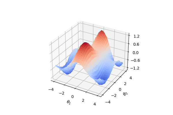
Cost function surface for circuit ansatz

Now, we plot the cost function surface for later comparison with the surface generated by learning the circuit structure.

from matplotlib import cm
from matplotlib.ticker import MaxNLocator
from mpl_toolkits.mplot3d import Axes3D

fig = plt.figure(figsize=(6, 4))
ax = fig.add_subplot(projection="3d")

X = np.linspace(-4.0, 4.0, 40)
Y = np.linspace(-4.0, 4.0, 40)
xx, yy = np.meshgrid(X, Y)
Z = np.array([[cost([x, y]) for x in X] for y in Y]).reshape(len(Y), len(X))
surf = ax.plot_surface(xx, yy, Z, cmap=cm.coolwarm, antialiased=False)

ax.set_xlabel(r"$\theta_1$")
ax.set_ylabel(r"$\theta_2$")
ax.zaxis.set_major_locator(MaxNLocator(nbins=5, prune="lower"))

plt.show()

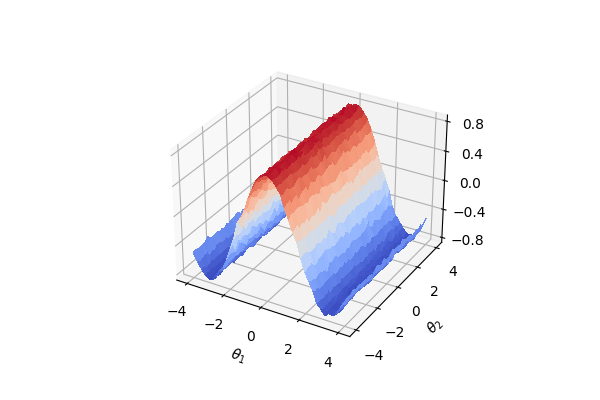
It is apparent that, based on the circuit structure chosen above, the cost function does not depend on the angle parameter \(\theta_2\) for the rotation gate \(R_y\). As we will show in the following sections, this independence is not true for alternative gate choices.

Rotoselect

We now implement the Rotoselect algorithm to learn a good selection of gates to minimize our cost function. The structure is similar to the original ansatz, but the generators of rotation are selected from the set of Pauli gates \(P_d \in \{X,Y,Z\}\) as shown in the figure above. For example, \(U(\theta,Z) = R_z(\theta)\).

Creating a quantum circuit with variable gates

First, we set up a quantum circuit with a similar structure to the one above, but instead of fixed rotation gates \(R_x\) and \(R_y\), we allow the gates to be specified with the generators keyword, which is a list of the generators of rotation that will be used for the gates in the circuit. For example, generators=['X', 'Y'] reproduces the original circuit ansatz used in the Rotosolve example above. A helper method RGen returns the correct unitary gate according to the rotation specified by an element of generators.

def RGen(param, generator, wires):
    if generator == "X":
        qml.RX(param, wires=wires)
    elif generator == "Y":
        qml.RY(param, wires=wires)
    elif generator == "Z":
        qml.RZ(param, wires=wires)


def ansatz_rsel(params, generators):
    RGen(params[0], generators[0], wires=0)
    RGen(params[1], generators[1], wires=1)
    qml.CNOT(wires=[0, 1])


@qml.qnode(dev)
def circuit_rsel(params, generators):
    ansatz_rsel(params, generators)
    return qml.expval(qml.PauliZ(0)), qml.expval(qml.PauliY(1))


@qml.qnode(dev)
def circuit_rsel2(params, generators):
    ansatz_rsel(params, generators)
    return qml.expval(qml.PauliX(0))


def cost_rsel(params, generators):
    Z_1, Y_2 = circuit_rsel(params, generators)
    X_1 = circuit_rsel2(params, generators)
    return 0.5 * Y_2 + 0.8 * Z_1 - 0.2 * X_1

Helper methods

We define helper methods in a similar fashion to Rotosolve. In this case, we must iterate through the possible gate choices in addition to optimizing each parameter.

def rotosolve(d, params, generators, cost, M_0):  # M_0 only calculated once
    params[d] = np.pi / 2.0
    M_0_plus = cost(params, generators)
    params[d] = -np.pi / 2.0
    M_0_minus = cost(params, generators)
    a = np.arctan2(
        2.0 * M_0 - M_0_plus - M_0_minus, M_0_plus - M_0_minus
    )  # returns value in (-pi,pi]
    params[d] = -np.pi / 2.0 - a
    if params[d] <= -np.pi:
        params[d] += 2 * np.pi
    return cost(params, generators)


def optimal_theta_and_gen_helper(d, params, generators, cost):
    params[d] = 0.0
    M_0 = cost(params, generators)  # M_0 independent of generator selection
    for generator in ["X", "Y", "Z"]:
        generators[d] = generator
        params_cost = rotosolve(d, params, generators, cost, M_0)
        # initialize optimal generator with first item in list, "X", and update if necessary
        if generator == "X" or params_cost <= params_opt_cost:
            params_opt_d = params[d]
            params_opt_cost = params_cost
            generators_opt_d = generator
    return params_opt_d, generators_opt_d


def rotoselect_cycle(cost, params, generators):
    for d in range(len(params)):
        params[d], generators[d] = optimal_theta_and_gen_helper(d, params, generators, cost)
    return params, generators

Optimizing the circuit structure

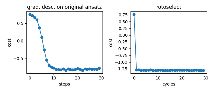
We perform the optimization and print the optimal generators for the rotation gates. The minimum value of the cost function obtained by optimizing using Rotoselect is less than the minimum value of the cost function obtained by gradient descent or Rotosolve, which were performed on the original circuit structure ansatz. In other words, Rotoselect performs better without increasing the depth of the circuit by selecting better gates for the task of minimizing the cost function.

costs_rsel = []
params_rsel = init_params.copy()
init_generators = np.array(["X", "Y"], requires_grad=False)
generators = init_generators
for _ in range(n_steps):
    costs_rsel.append(cost_rsel(params_rsel, generators))
    params_rsel, generators = rotoselect_cycle(cost_rsel, params_rsel, generators)

print("Optimal generators are: {}".format(generators.tolist()))

# plot cost function vs. steps comparison
fig, (ax1, ax2) = plt.subplots(1, 2, figsize=(7, 3))
plt.subplot(1, 2, 1)
plt.plot(steps, costs_gd, "o-")
plt.title("grad. desc. on original ansatz")
plt.xlabel("steps")
plt.ylabel("cost")
plt.subplot(1, 2, 2)
plt.plot(steps, costs_rsel, "o-")
plt.title("rotoselect")
plt.xlabel("cycles")
plt.ylabel("cost")
plt.yticks(np.arange(-1.25, 0.80, 0.25))
plt.tight_layout()
plt.show()

Out:

Optimal generators are: ['Y', 'X']

Cost function surface for learned circuit structure

Finally, we plot the cost function surface for the newly discovered optimized circuit structure shown in the figure above. It is apparent from the minima in the plot that the new circuit structure is better suited for the problem.

fig = plt.figure(figsize=(6, 4))
ax = fig.add_subplot(projection="3d")

X = np.linspace(-4.0, 4.0, 40)
Y = np.linspace(-4.0, 4.0, 40)
xx, yy = np.meshgrid(X, Y)
# plot cost for fixed optimal generators
Z = np.array([[cost_rsel([x, y], generators) for x in X] for y in Y]).reshape(
    len(Y), len(X)
)
surf = ax.plot_surface(xx, yy, Z, cmap=cm.coolwarm, antialiased=False)

ax.set_xlabel(r"$\theta_1$")
ax.set_ylabel(r"$\theta_2$")
ax.zaxis.set_major_locator(MaxNLocator(nbins=5, prune="lower"))

plt.show()

References

1. Mateusz Ostaszewski, Edward Grant, Marcello Bendetti. “Quantum circuit structure learning.” arxiv:1905.09692, 2019.

About the author

Angus Lowe

Angus is currently a PhD student in physics at the Massachusetts Institute of Technology. His main research interests are in the theory of quantum computation and quantum information.

demos/tutorial_rotoselect

 

Download Python script

 

Download Notebook

 

View on GitHub