Quantum computing with superconducting qubits

Author: Alvaro Ballon — Posted: 22 March 2022. Last updated: 26 August 2022.

Superconducting qubits are among the most promising approaches to building quantum computers. It is no surprise that this technology is being used by well-known tech companies in their quest to pioneer the quantum era. Google’s Sycamore claimed quantum advantage back in 2019 1 and, in 2021, IBM built its Eagle quantum computer with 127 qubits 2! The central insight that allows for these quantum computers is that superconductivity is a quantum phenomenon, so we can use superconducting circuits as quantum systems that we can control at will. We can actually bring the quantum world to a larger scale and manipulate it more freely!

By the end of this demo, you will learn how superconductors are used to create, prepare, control, and measure the state of a qubit. Moreover, you will identify the strengths and weaknesses of this technology in terms of Di Vincenzo’s criteria, as introduced in the box below. You will be armed with the basic concepts to understand the main scientific papers on the topic and keep up-to-date with the newest developments.

Di Vincenzo’s criteria: In the year 2000, David DiVincenzo proposed a wishlist for the experimental characteristics of a quantum computer 3. DiVincenzo’s criteria have since become the main guideline for physicists and engineers building quantum computers:

1. Well-characterized and scalable qubits. Many of the quantum systems that we find in nature are not qubits, so we must find a way to make them behave as such. Moreover, we need to put many of these systems together.

2. Qubit initialization. We must be able to prepare the same state repeatedly within an acceptable margin of error.

3. Long coherence times. Qubits will lose their quantum properties after interacting with their environment for a while. We would like them to last long enough so that we can perform quantum operations.

4. Universal set of gates. We need to perform arbitrary operations on the qubits. To do this, we require both single-qubit gates and two-qubit gates.

5. Measurement of individual qubits. To read the result of a quantum algorithm, we must accurately measure the final state of a pre-chosen set of qubits.

Superconductivity

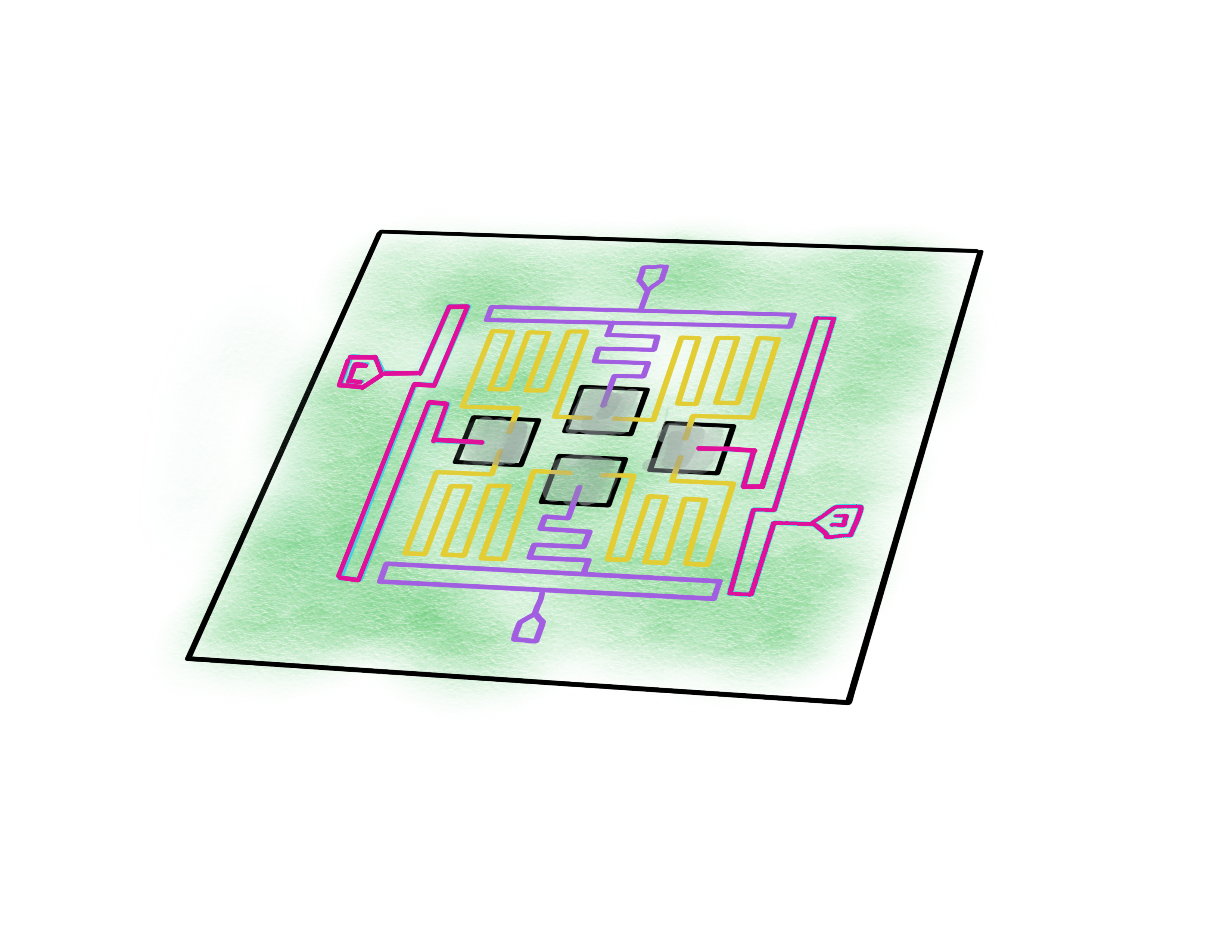
Superconducting chip with 4 qubits

To understand how superconducting qubits work, we first need to explain why some materials are superconductors. Let’s begin by addressing a simpler question: why do conductors allow for the easy passage of electrons and insulating materials don’t? Solid-state physics tells us that when an electric current travels through a material, the electrons therein come in two types. Conduction electrons flow freely through the material, while valence electrons are attached to the atoms that form the material itself. A material is a good conductor of electricity if the valence electrons require no energy to be stripped from the atoms to become conduction electrons. Similarly, the material is a semi-conductor if the energy needed is small, and it’s an insulator if the energy is large.

But, if conduction electrons can be obtained for free in conducting materials, then why don’t all conductors have infinite conductivity? Even the tiniest of stimuli should create a very large current! To address this valid concern, let us recall the exclusion principle in atomic physics: the atom’s discrete energy levels have a population limit, so only a limited number of electrons can have the same energy. However, the exclusion principle is not limited to electrons in atomic orbitals. In fact, it applies to all electrons that are organized in discrete energy levels. Since conduction electrons also occupy discrete conduction energy levels, they must also abide by this law! The conductivity is then limited because, when the lower conduction energy levels are occupied, the energy required to promote valence to conduction electrons is no longer zero. This energy will keep increasing as the population of conduction electrons grows.

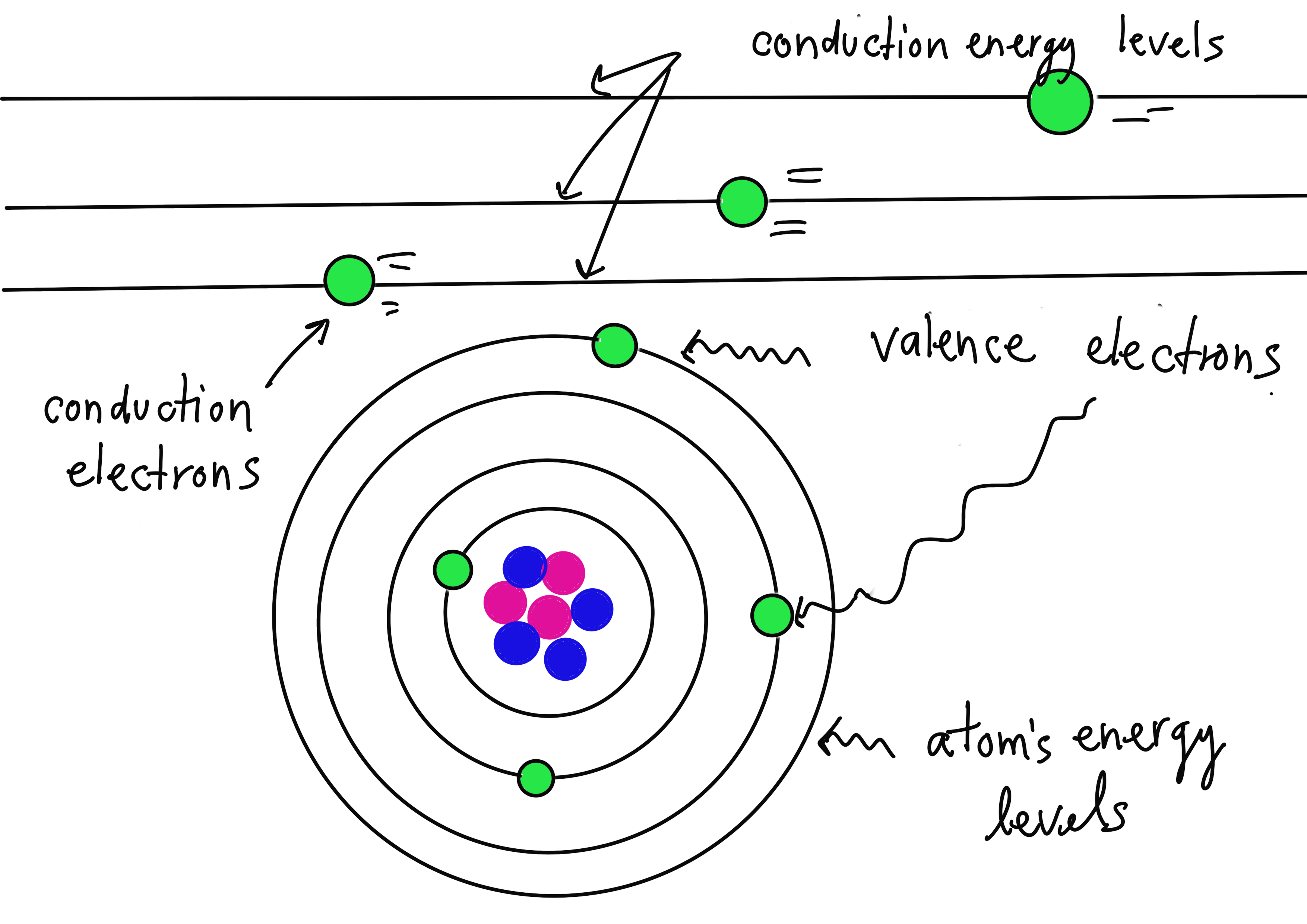
Valence and conduction energy levels

However, superconductors do have infinite conductivity. How is this even possible? It’s not a phenomenon that we see in our daily lives. For some materials, at extremely low temperatures, the conduction electrons attract the positive nuclei to form regions of high positive charge density, alternating with regions of low charge density. This charge distribution oscillates in an organized manner, creating waves in the material known as phonons. The conduction electrons are pushed together by these phonons, forming Cooper pairs. Most importantly, these coupled electrons need not obey the exclusion principle. We no longer have an electron population limit in the lower conduction energy levels, allowing for infinite conductivity! 4

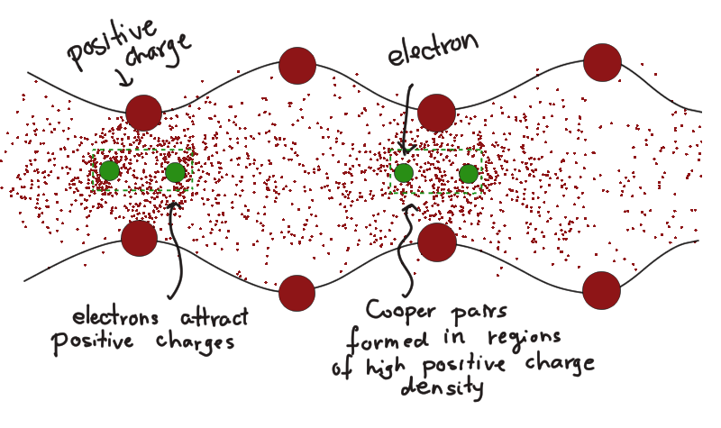
Cooper pairs are formed by alternating regions of high and low density of positive charge (phonons) represented by the density of red dots.

PennyLane plugins: You can run your quantum algorithms on actual superconducting qubit quantum computers on the Cloud. The Qiskit, Amazon Braket, Cirq, and Rigetti PennyLane plugins give you access to some of the most powerful superconducting quantum hardware.

Building an artificial atom

When we code in PennyLane, we deal with the abstraction of a qubit. But how is a qubit actually implemented physically? Some of the most widely used real-life qubits are built from individual atoms. But atoms are given to us by nature, and we cannot easily alter their properties. So although they are reliable qubits, they are not very versatile. We may adapt our technology to the atoms, but they seldom adapt to our technology. Could there be a way to build a device with the same properties that make atoms suitable qubits? Let’s see if we can build an artificial atom!

Our first task is to isolate the features that an ideal qubit should have. First and foremost, we must not forget that a qubit is a physical system with two distinguishable configurations that correspond to the computational basis states. In the case of an atom, these are usually the ground and excited states, \(\left\lvert g \right\rangle\) and \(\left\lvert e \right\rangle\), of a valence electron. In atoms, we can distinguish these states reliably because the ground and excited states have two distinct values of energy that can be resolved by our measuring devices. If we measure the energy of the valence electron that is in either \(\left\lvert g \right\rangle\) or \(\left\lvert e \right\rangle\), we will measure two — and only two — possible values \(E_0\) and \(E_1\), associated to \(\left\lvert g \right\rangle\) and \(\left\lvert e \right\rangle\) respectively.

Most importantly, the physical system under consideration must exhibit quantum properties. The presence of discrete energy levels is indeed one such property, so if we do build a device that stores energy in discrete values, we can suspect that it obeys the laws of quantum mechanics. Usually, one thinks of a quantum system as being at least as small as a molecule, but building something so small is technologically impossible. It turns out that we don’t need to go to such small scales. If we build a somewhat small electric circuit using superconducting wires and bring it to temperatures of about 10 mK, it becomes a quantum system with discrete energy levels.

Finally, we must account for the fact that electrons in atoms have more states available than just \(\left\lvert g \right\rangle\) and \(\left\lvert e \right\rangle\). In fact, the energy levels in an atom are infinitely many. How do we guarantee that an electron does not escape to another state that is neither of our hand-picked states? The transition between the ground and the excited state only happens when the electron absorbs a photon (a particle of light) with energy \(\Delta E = E_1 - E_0\). To get to another state with energy \(E_2\), the electron would need to absorb a photon with energy \(E_2 - E_1\) or \(E_2-E_0\). In an atom, these energy differences are always different: there is a non-uniform spacing between the energy levels. Therefore, if we limit ourselves to interacting with the atom using photons with energy \(\Delta E\), we will not go beyond the states that define our qubit.

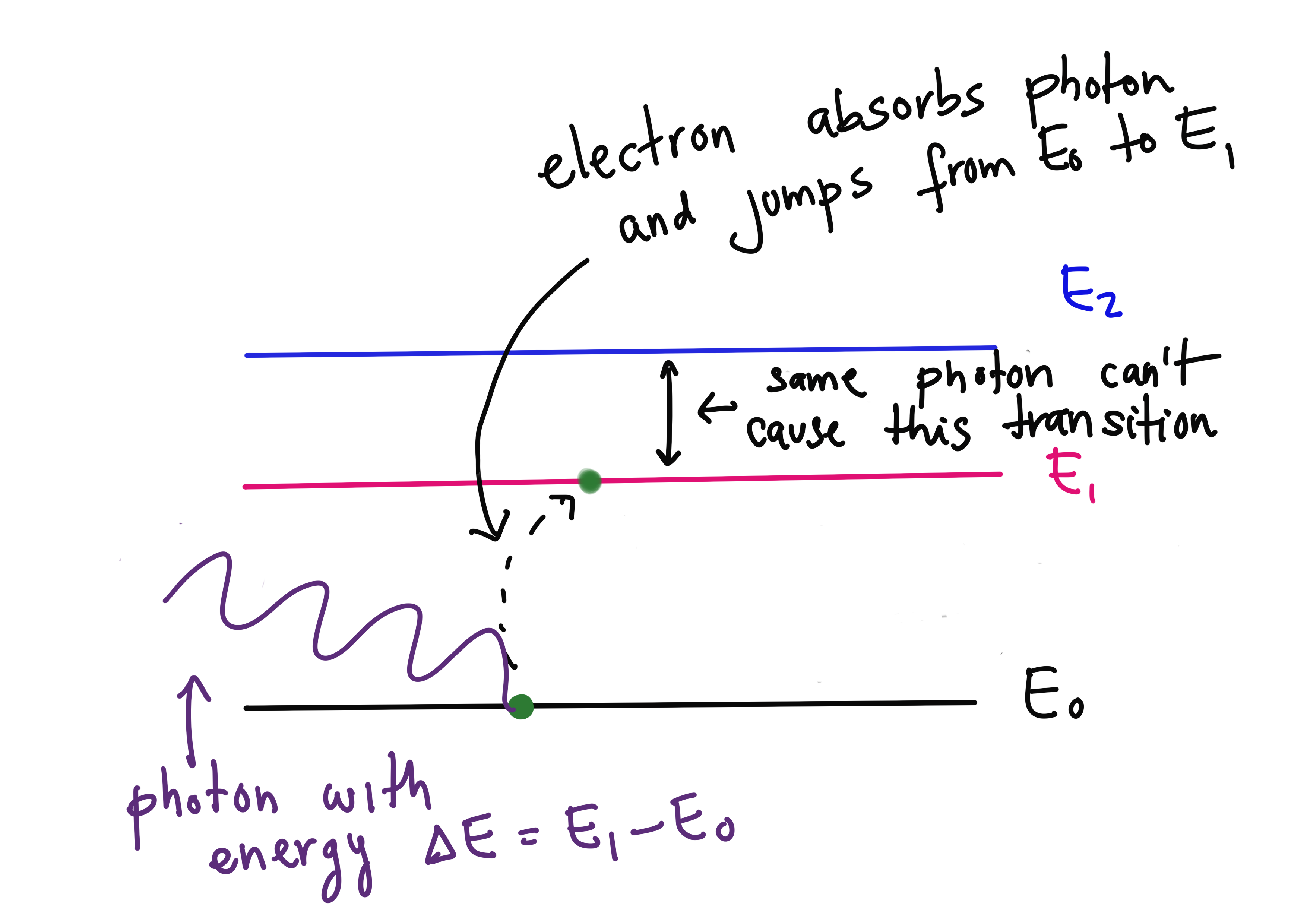
Photons with a particular energy excite electrons

Let’s then build the simplest superconducting circuit. We do not want the circuit to warm up, or it will lose its quantum properties. Of all the elements that an ordinary circuit may have, only two do not produce heat when they’re superconducting: capacitors and inductors. Capacitors are two parallel metallic plates that store electric charge. They are characterized by their capacitance \(C\), which measures how much charge they can store when connected to a given power source. Inductors are wires shaped as a coil and store magnetic fields when a current passes through. These magnetic fields, in turn, slow down changing currents that pass through the inductor. They are described by an inductance \(L\), which measures the strength of the magnetic field stored in the inductor at a fixed current. The simplest superconducting circuit is, therefore, a capacitor connected to an inductor, also known as an LC circuit, as shown below:

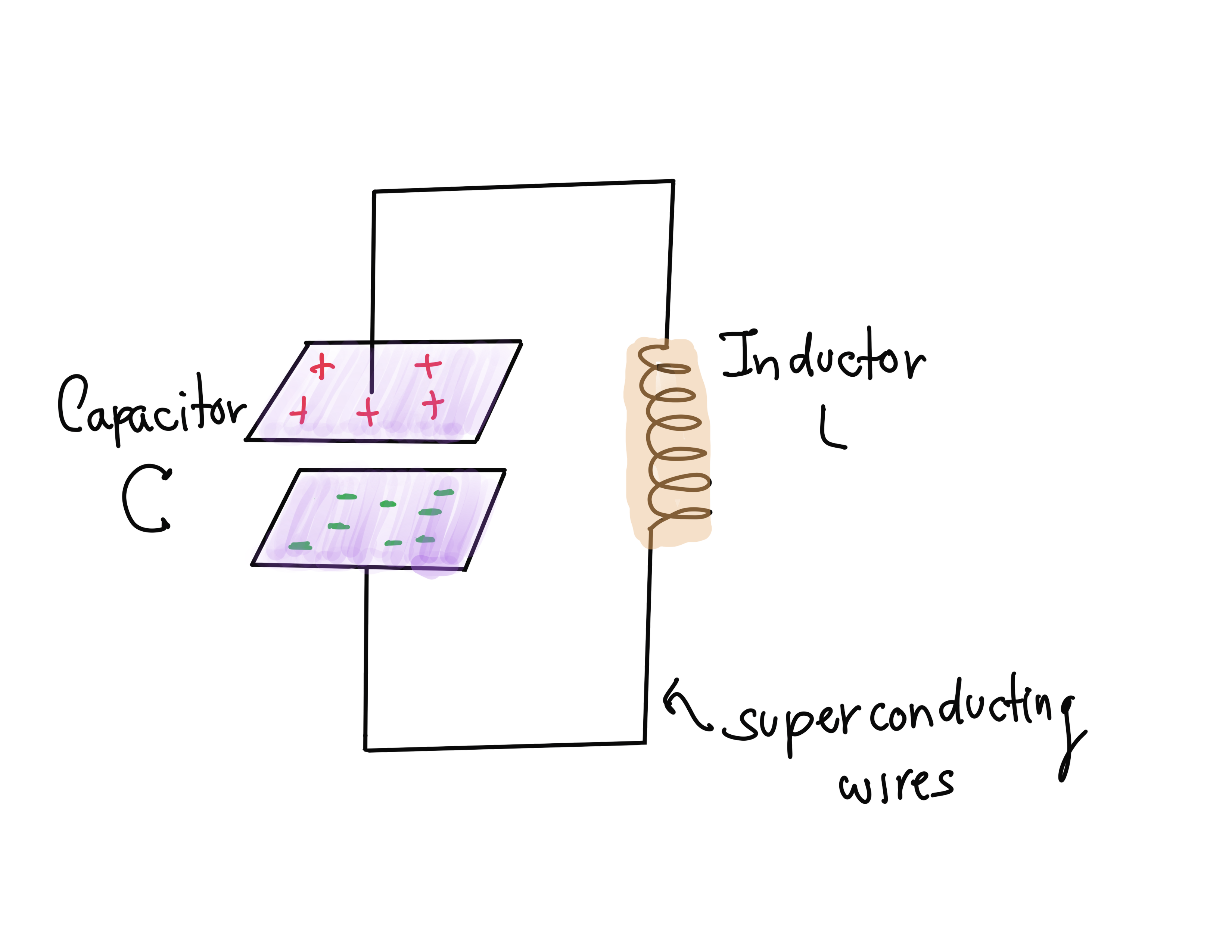
Superconducting LC circuit

Sadly, this simple circuit has a problem: the spacing between energy levels is constant, which means identical photons will cause energy transitions between many neighbouring pairs of states. This makes it impossible to isolate just two specific states for our qubit.

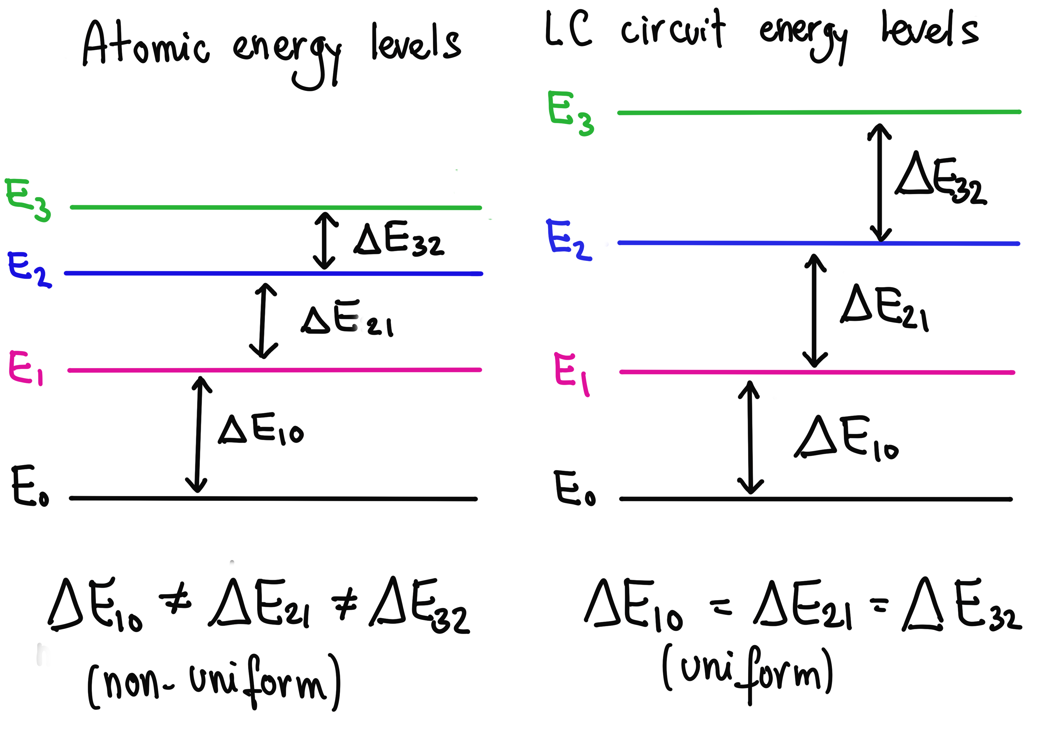
Non-uniform energy levels in an atom vs. uniform energy levels in a superconducting LC circuit

But there turns out to be a fix for the even spacing. Enter the Josephson junction. It consists of a very thin piece of an insulating material placed between two superconducting metals. Why do we need this? If it’s insulating, no current should go through it and our circuit should stop working! Here’s where another famous quantum effect comes into play: the tunnel effect. Due to the quantum-probabilistic behaviour of their location, Cooper pairs can sometimes go through the Josephson junction, so that the current is reduced but not completely stopped. If we replace the inductor with one of these junctions, the energy levels of the superconducting circuit become unevenly spaced, exactly as we wanted. We have built an artificial atom!

The transmon

Mission accomplished? Not yet. We want our qubit to be useful for building quantum computers. In short, this means that we need to interact with the environment in a controlled way. A way to do this is to add a gate capacitor with capacitance \(C_g\) to the artificial atom, so that it can receive external signals (photons, in our case). The amount of charge \(Q_g\) in this capacitor can be chosen by the operator, and it determines how strongly the circuit interacts with the environment.

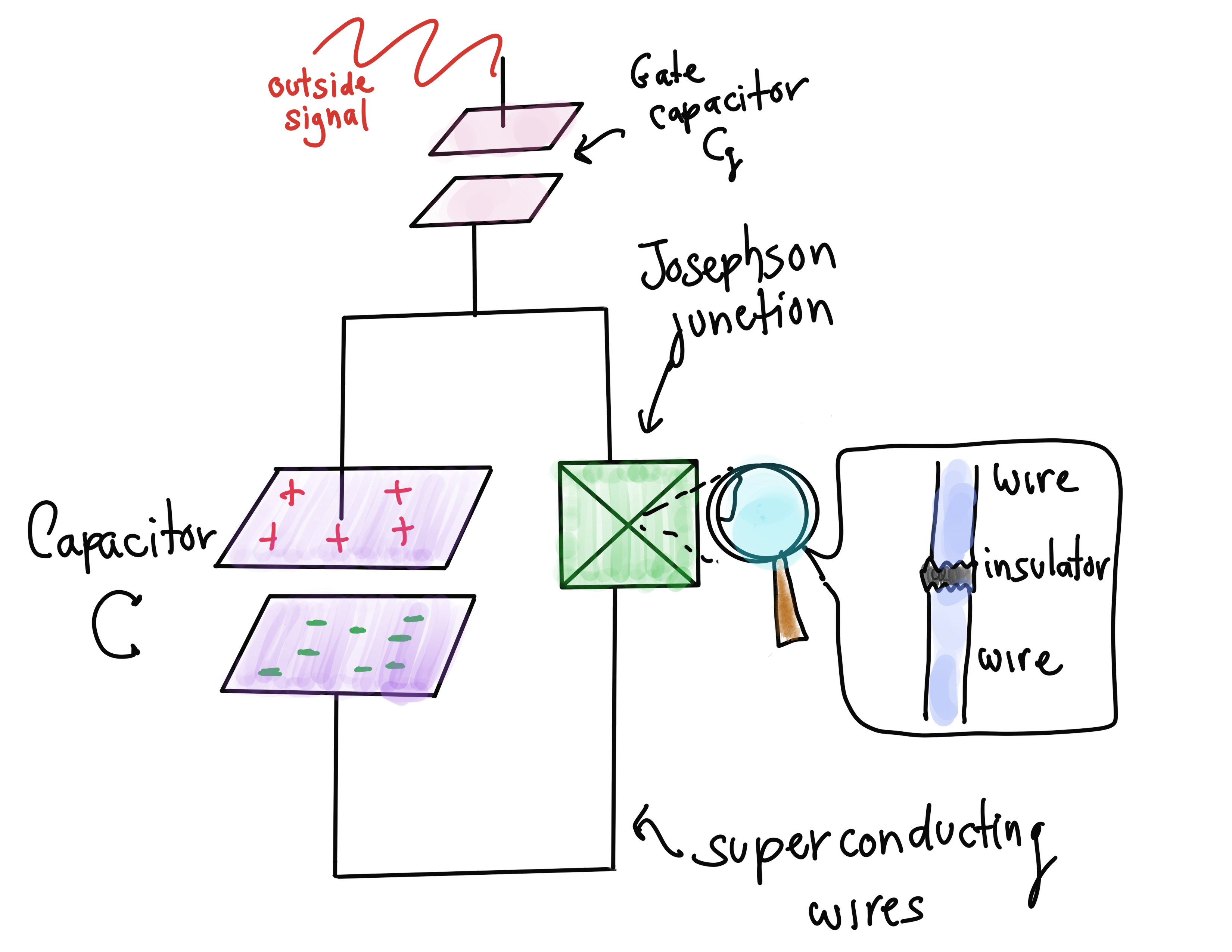
Circuit with a Josephson junction and a gate capacitor

But we run into a problem again. Adding a gate capacitor messes with our uneven energy levels, which we worked so hard to obtain. The separation in energy levels depends on \(Q_g,\) as shown below 5.

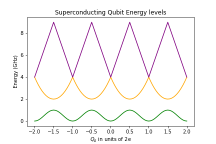
First three energy levels (green, orange, purple) as a function of the charge in the gate capacitor.

The problem with this dependence is that a small change in the gate charge \(Q_g\) can change the difference in energy levels significantly. A solution to this issue is to work around the value \(Q_g/2e = 1/2\), where the levels are not too sensitive to changes in the gate charge. But there is a more straightforward solution: the difference in energy levels also depends on the in-circuit capacitance \(C\) and the physical characteristics of the junction. If we can make the capacitance larger, the energy level differences become less sensitive to \(Q_g\). So all we need to do is choose an appropriate capacitor.

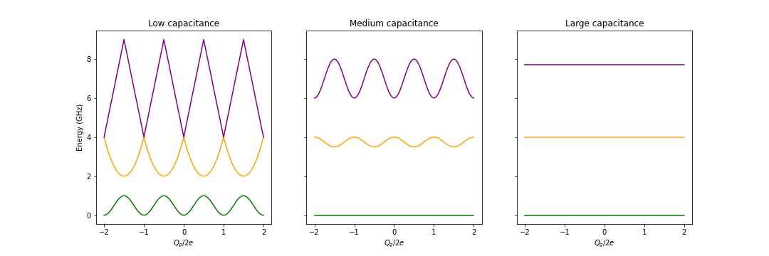
Energy levels vs gate capacitor charge for different values of in-circuit capacitance.

But there is a price to be paid: making the in-circuit capacitance \(C\) larger does reduce the sensitivity to the gate charge, but it also makes the differences in energy levels more uniform. Does that make the Josephson junction pointless? Thankfully, the latter effect turns out to be smaller than the former, so we can adjust the capacitance value and preserve some non-uniformity. The regime that has been proven ideal is known as the transmon regime, and artificial atoms in this regime are called transmons. They have proven to be highly effective as qubits, and they are used in many applications nowadays. We can thus work with the first two energy levels of the transmon, which we will also denote \(\left\lvert g \right\rangle\) and \(\left\lvert e \right\rangle\), the ground and excited states respectively. The energy difference between these states is known as the energy gap \(E_a\). We can stimulate transitions using photons of frequency \(\omega_a\), where

\[E_a = \hbar\omega_a.\]

We have now partially satisfied Di Vincenzo’s first criterion of a well-defined qubit, and we will discuss scalability later. A great feature of superconducting qubits is that the second criterion is satisfied effortlessly. Since the excited states in an artificial atom are short-lived and prefer to be on the ground state, all we have to do is wait for a short period. If the circuit is well isolated, it is guaranteed that all the qubits will be in the ground state with a high probability after this short interval.

Measuring the circuit’s state

Now that we have finally fabricated our qubit, we need to understand how to manipulate it. The way to do this is to put the qubit inside an optical cavity, a metal box where we can contain electromagnetic waves. Our focus will be on the so-called Fabry-Perot cavities. They consist of two mirrors facing each other and whose rears are coated with an anti-reflecting material. Something surprising happens when we shine a beam of light on a Fabry-Perot cavity of length \(L\): electromagnetic waves will only be transmitted when they have a wavelength \(\lambda\) such that

\[L = n\lambda/2,\]

where \(n\) is an arbitrary positive integer. If this condition is not met, most of the photons in the wave will be reflected away. Therefore, we will have an electromagnetic field inside if we carefully tune our light source to one of these wavelengths. For superconducting qubits, it is most common to use wavelengths in the microwave range.

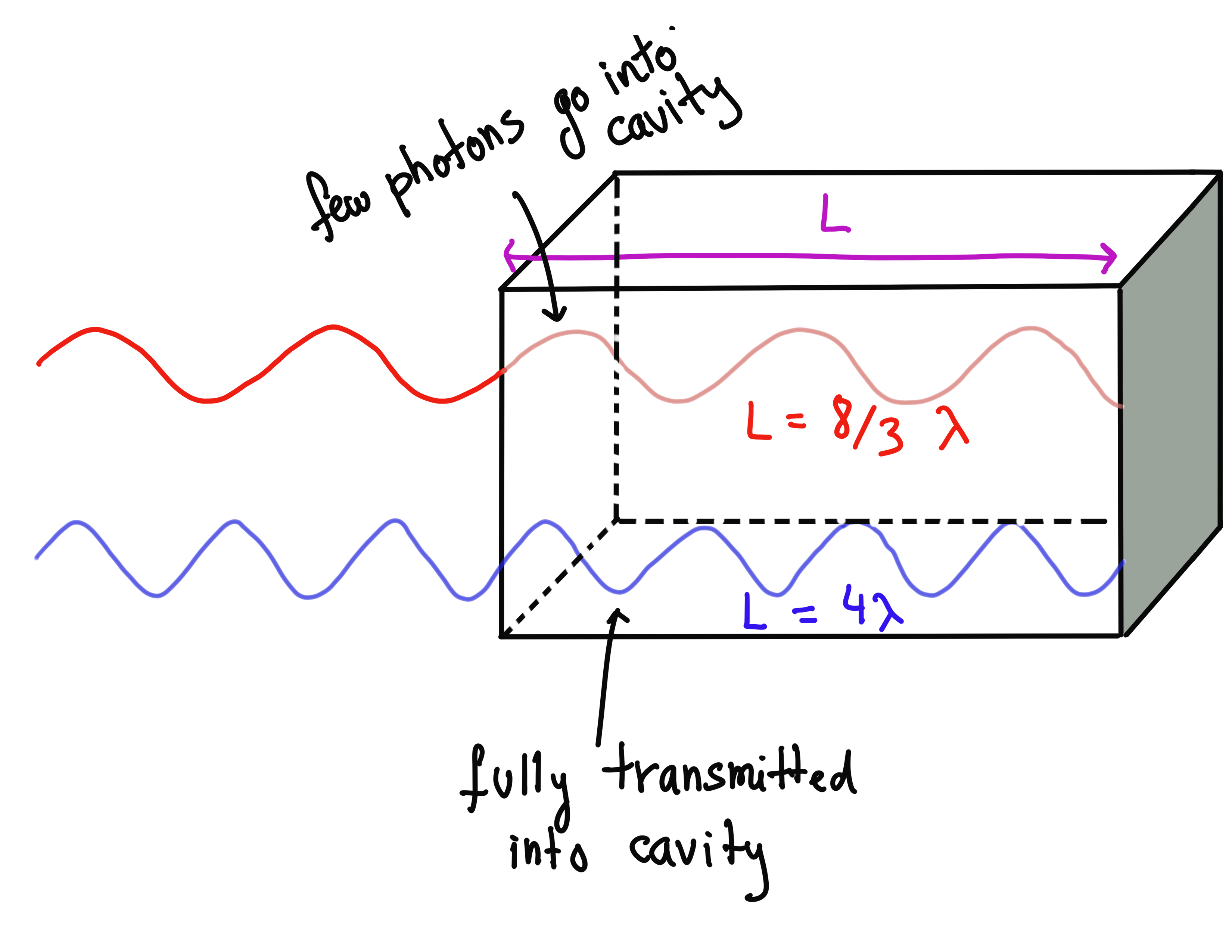
The Fabry-Perot Cavity rejects most of the red wave but allows all of the blue wave, since an integer number of blue wavelengths fit exactly in the cavity.

Following Di Vincenzo’s fifth criterion, let’s see how we can measure the state of the qubit placed inside the cavity. To obtain information, we need to shine light at a frequency \(\omega_r\) that the cavity lets through (recall that the frequency and the wavelength are related via \(\omega = 2\pi c/\lambda\), where \(c\) is the speed of light). We may also choose the frequency value \(\omega_r\) to be far from the transmon’s frequency gap \(\omega_a\), so the qubit does not absorb the photons. Namely, the detuning \(\Delta\) needs to be large:

\[\Delta \equiv \left\lvert \omega_r - \omega_a \right\rvert \gg 1.\]

What happens to the photons of this frequency that meet paths with the qubit? They are scattered by the circuit, as opposed to photons of frequency \(\omega_a\), which get absorbed. Scattering counts as an interaction, albeit a weak one, so the scattered photons contain some information about the qubit’s state. Indeed, the collision causes an exchange in momentum and energy. For light, this means that its amplitude and phase will change slightly. If we carefully measure the properties of the scattered light, we can distill the information about the state of the qubit and measure its state.

To understand how this works in more detail, we need to do some hands-on calculations. We will rely on the concept of a Hamiltonian; do read the blue box below if you need a refresher on the topic!

Primer on Hamiltonians: When a physical system is exposed to outside influences, it will change configurations. One way to describe these external interactions is through a mathematical object called a Hamiltonian, which represents the total energy on the system. In quantum mechanics, the Hamiltonian \(\hat{H}\) is a Hermitian matrix whose eigenvalues represent the possible energies the system may have. The Hamiltonian also tells us how an initial state changes in time. In quantum mechanics, this change is described by a differential equation known as Schrodinger’s equation:

\[i\hbar \frac{\partial}{\partial t}\left\lvert \psi(t)\right\rangle = \hat{H}\left\lvert \psi(t)\right\rangle.\]

When the Hamiltonian does not depend on time, this equation can be solved exactly:

\[\left\lvert \psi(t)\right\rangle= \exp(-i\hat{H}t/\hbar)\left\lvert \psi(0)\right\rangle\]

where \(\exp\) represents the matrix exponential. Don’t worry, there’s no need to know how to solve this equation or calculate matrix exponentials. Pennylane can do this for us using ApproxTimeEvolution.

We are given a Hamiltonian \(\hat{H}\) that describes the transmon and the photons inside the cavity. The transmon is initially in its ground state \(\left\lvert g \right\rangle,\) and the cavity starts without any photons in it, i.e., in the vacuum state denoted by \(\left\lvert 0 \right\rangle\). According to Schrodinger’s equation, the state of the cavity (transmon and photons system) evolves into \(\left\lvert \psi(t)\right\rangle= \exp(-i\hat{H}t/\hbar)\left\lvert g \right\rangle\left\lvert 0 \right\rangle\) after a time \(t\). What is the Hamiltonian that describes light of amplitude \(\epsilon\) and frequency \(\omega_r\) incident on the cavity, when the detuning \(\Delta\) is large? Deriving the Hamiltonian is not an easy job, so we should trust physicists on this one! The Hamiltonian turns out to be

\[\hat{H}=\hbar(\omega_r I+\chi\hat{\sigma}_z)\otimes\hat{N} + \hbar\epsilon I\otimes \hat{P},\]

where \(\hat{N}\) counts the number of photons in the cavity, \(\hat{P}\) is the photon momentum operator, and \(\epsilon\) is the amplitude of the electromagnetic wave incident on the cavity. The shift \(\chi\) is a quantity that depends on the circuit and gate capacitances and the detuning \(\Delta\).

The effect of this evolution can be calculated explicitly. Shining microwaves on the cavity gives us a coherent state of light contained in it, which is the state of light that lasers give out. Coherent states are completely determined by two quantities called \(\bar{x}\) and \(\bar{p}\) (these quantities are mathematically similar to the notions of average position and average momentum, but are in fact physically connected to the phase of the light), so we will denote them via \(\left\lvert \bar{x}, \bar{p}\right\rangle\). For the state of the qubit and cavity system, we write the ket in the form \(\left\lvert g \right\rangle \left\lvert \bar{x}, \bar{p}\right\rangle\). The Hamiltonian above has (approximately) the following effect:

\[\left\lvert g \right\rangle \left\lvert 0 \right\rangle \rightarrow \left\lvert g \right\rangle \left\lvert \epsilon t, (\omega_r+\chi)t \right\rangle,\]

\[\left\lvert e \right\rangle \left\lvert 0 \right\rangle \rightarrow \left\lvert e \right\rangle \left\lvert \epsilon t, (\omega_r-\chi)t \right\rangle.\]

Consequently, if the state of the qubit was initially the superposition \(\alpha \left\lvert g \right\rangle +\beta \left\lvert e \right\rangle\), then the qubit-cavity system would evolve to the state

\[\left\lvert\psi(t)\right\rangle=\alpha \left\lvert g \right\rangle \left\lvert \epsilon t, (\omega_r+\chi)t \right\rangle +\beta \left\lvert e \right\rangle \left\lvert \epsilon t, (\omega_r-\chi)t \right\rangle.\]

In general, this state represents an entangled state between the qubit and the cavity. So if we measure the state of the light trapped by the cavity, we can determine the qubit’s state as well.

Let us see how this works in practice using PennyLane. The default.gaussian device allows us to simulate coherent states of light. These states start implicitly in the vacuum (no photons) state. The PennyLane function qml.Displacement(x,0) applies a displacement operator, which creates a coherent state \(\left\lvert \bar{x}, 0\right\rangle\). The rotation operator qml.Rotation(phi) rotates the state \(\left\lvert \bar{x}, 0\right\rangle\) in \((x, p)\) space. When applied after a large displacement, it changes the value of \(\bar{x}\) only slightly, but noticeably changes the value of \(\bar{p}\) by shifting it off from zero, as shown in the figure 5:

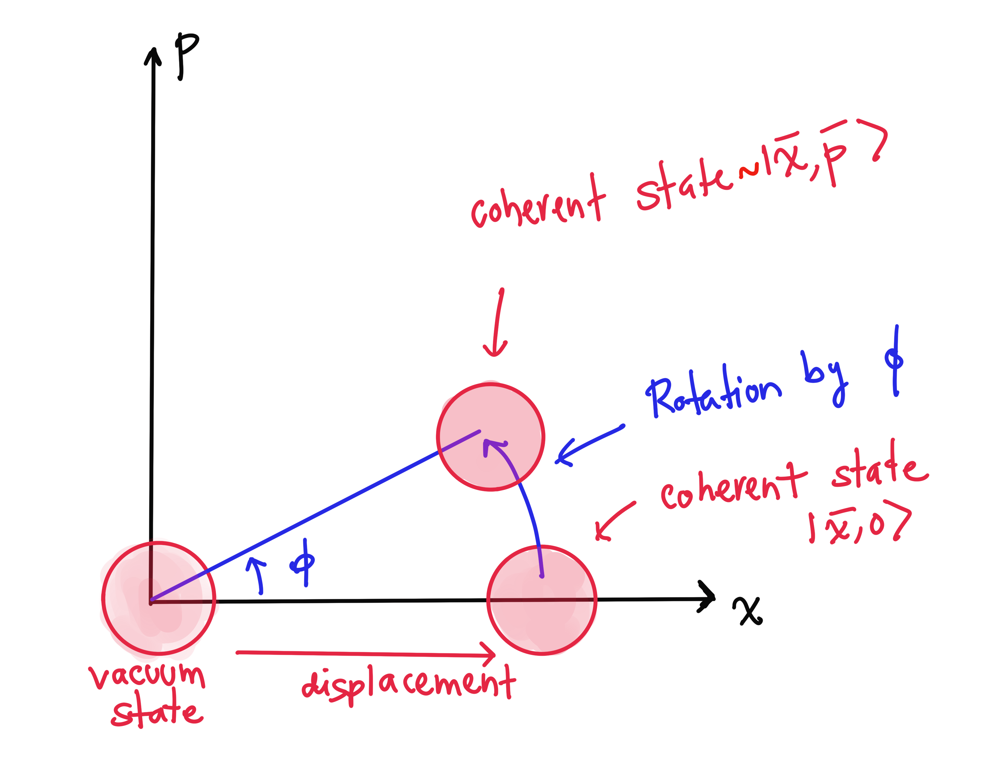
Translation and rotation in the position-momentum picture

It turns out that this sequence of operations implements the evolution of the cavity state exactly. Note that here we are taking \(\omega_r=0\), which simply corresponds to taking \(\omega_r\) as a reference frequency, so a rotation by angle \(\phi\) actually means a rotation by \(\omega_r+\phi\). In PennyLane, the operations read:

import pennylane as qml
from pennylane import numpy as np
import matplotlib.pyplot as plt

# Call the default.gaussian device with 50 shots
dev = qml.device("default.gaussian", wires=1, shots=50)

# Fix parameters
epsilon, chi = 1.0, 0.1

# Implement displacement and rotation and measure both X and P observables


@qml.qnode(dev, interface="autograd")
def measure_P_shots(time, state):
    qml.Displacement(epsilon * time, 0, wires=0)
    qml.Rotation((-1) ** state * chi * time, wires=0)
    return qml.sample(qml.P(0))


@qml.qnode(dev, interface="autograd")
def measure_X_shots(time, state):
    qml.Displacement(epsilon * time, 0, wires=0)
    qml.Rotation((-1) ** state * chi * time, wires=0)
    return qml.sample(qml.X(0))

Note

It may be surprising to see the default.gaussian device being used here, since it is most often used when we work with photonic systems. But it is also valid to use it here, since we are modelling a measurement process that uses photons.

We measure the photon’s momentum at the end, since it allows us to distinguish qubit states as long as we can resolve them. Let us plot for three different durations of the microwave-cavity interaction. We will simulate the measurement of 50 photons, which can inform us whether the qubit is in the ground or excited state:

fig, (ax1, ax2, ax3) = plt.subplots(1, 3, figsize=(15, 5))
fig.suptitle("Position/momentum measurement", fontsize=18)
ax1.scatter(measure_X_shots(1, 0), measure_P_shots(1, 0))
ax1.scatter(measure_X_shots(1, 1), measure_P_shots(1, 1))
ax2.scatter(measure_X_shots(3, 0), measure_P_shots(3, 0))
ax2.scatter(measure_X_shots(3, 1), measure_P_shots(3, 1))
ax3.scatter(measure_X_shots(5, 0), measure_P_shots(5, 0))
ax3.scatter(measure_X_shots(5, 1), measure_P_shots(5, 1))
ax1.set_title(r"$t=1/\epsilon$", fontsize=16)
ax2.set_title(r"$t=3/\epsilon$", fontsize=16)
ax3.set_title(r"$t=5/\epsilon$", fontsize=16)
ax1.set_ylabel("Momentum", fontsize=16)
ax2.set_xlabel("Position", fontsize=16)
plt.show()

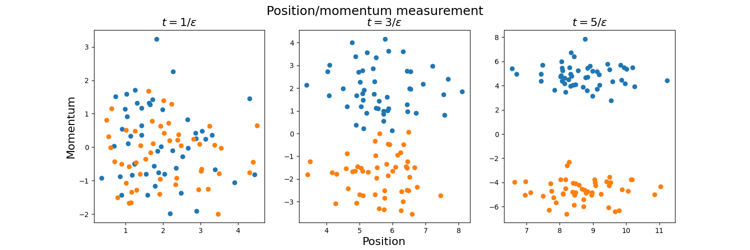
In the above, the blue and orange dots represent qubits which we can infer to be in the state \(\left\lvert g \right\rangle\) and \(\left\lvert e \right\rangle\) respectively.

We see that the longer we shine microwaves on the cavity, the greater our ability to resolve the momentum change, making for an equally good measurement of the qubit’s state. However, this poses a problem: being a relatively large object, the state of the qubit is rather short-lived due to decoherence. Therefore, taking a long time to make the measurement introduces additional inaccuracies: the qubits may lose quantum properties due to decoherence before we even finish measuring! An outstanding challenge for superconducting qubit technologies is to perform measurements as fast as possible, in times well below the decoherence time.

Superconducting single-qubit gates

We have seen that shining light with detuning \(\Delta \gg 1\) is used to perform indirect measurements. A rather different choice, \(\omega_r =\omega_a\) (\(\Delta=0\)), allows us to manipulate the state of the qubit. But does the Fabry-Perot cavity transmit these photons if their wavelength does not allow it? We must emphasize that the cavity reflects only the vast majority of photons, but not all of them. If we compensate by increasing the radiation intensity, some photons will still be transmitted into the cavity and be absorbed by the superconducting qubit.

If we shine a coherent state light with frequency \(\omega_a\) on the cavity and phase \(\phi\) at the position of the qubit, then the Hamiltonian for the artificial atom is

\[\hat{H}=\hbar\Omega_R(\hat{\sigma}_{x}\cos\phi + \hat{\sigma}_{y}\sin\phi).\]

Here, \(\Omega_R\) is a special frequency called the Rabi frequency, which depends on the average electric field in the cavity and the size of the superconducting qubit. With this Hamiltonian, we can implement a universal set of single-qubit gates since \(\phi=0\) implements an \(X\)-rotation and \(\phi=\pi/2\) applies a \(Y\)-rotation.

Let us check this using PennyLane. For qubits, we can define Hamiltonians using qml.Hamiltonian and evolve an initial state using ApproxTimeEvolution:

from pennylane.templates import ApproxTimeEvolution

dev2 = qml.device("default.qubit", wires=1)

# Implement Hamiltonian evolution given phase phi and time t, from a given initial state
@qml.qnode(dev2, interface="autograd")
def H_evolve(state, phi, time):

    if state == 1:
        qml.PauliX(wires=0)

    coeffs = [np.cos(phi), np.sin(phi)]
    ops = [qml.PauliX(0), qml.PauliY(0)]
    Ham = qml.Hamiltonian(coeffs, ops)
    ApproxTimeEvolution(Ham, time, 1)
    return qml.state()


# Implement X rotation exactly
@qml.qnode(dev2, interface="autograd")
def Sc_X_rot(state, phi):

    if state == 1:
        qml.PauliX(wires=0)

    qml.RX(phi, wires=0)
    return qml.state()


# Implement Y rotation exactly
@qml.qnode(dev2, interface="autograd")
def Sc_Y_rot(state, phi):

    if state == 1:
        qml.PauliX(wires=0)

    qml.RY(phi, wires=0)
    return qml.state()


# Print to compare results

print("State |0>:")

print(
    "X-rotated by pi/3: {}; Evolved for phi=0, t=pi/6: {}".format(
        Sc_X_rot(0, np.pi / 3).round(2), H_evolve(0, 0, np.pi / 6).round(2)
    )
)
print(
    "Y-rotated by pi/3: {}; Evolved for phi=pi/2, t=pi/6: {}\n".format(
        Sc_Y_rot(0, np.pi / 3).round(2), H_evolve(0, np.pi / 2, np.pi / 6).round(2)
    )
)

print("State |1>:")
print(
    "X-rotated by pi/3: {}; Evolved for phi=0, t=pi/6: {}".format(
        Sc_X_rot(1, np.pi / 3).round(2), H_evolve(1, 0, np.pi / 6).round(2)
    )
)
print(
    "Y-rotated by pi/3: {}; Evolved for phi=pi/2, t=pi/6: {}\n".format(
        Sc_Y_rot(1, np.pi / 3).round(2), H_evolve(1, np.pi / 2, np.pi / 6).round(2)
    )
)

Out:

State |0>:
X-rotated by pi/3: [0.87+0.j  0.  -0.5j]; Evolved for phi=0, t=pi/6: [0.87+0.j  0.  -0.5j]
Y-rotated by pi/3: [0.87+0.j 0.5 +0.j]; Evolved for phi=pi/2, t=pi/6: [0.87-0.j 0.5 -0.j]

State |1>:
X-rotated by pi/3: [0.  -0.5j 0.87+0.j ]; Evolved for phi=0, t=pi/6: [0.  -0.5j 0.87+0.j ]
Y-rotated by pi/3: [-0.5 +0.j  0.87+0.j]; Evolved for phi=pi/2, t=pi/6: [-0.5 -0.j  0.87+0.j]

Thus, for a particular choice of angle, we have verified that this Hamiltonian implements rotations around the X and Y axes. We can do this for any choice of angle, where we see that the time interval needed for a rotation by an angle \(\theta\) is \(t=2\theta/\Omega_R.\) This time can be controlled simply by turning the source of microwaves on and off.

The typical times in which a single-qubit gate is executed are in the order of the nanoseconds, making superconducting quantum computers the fastest ones out there. Why do they have this intrinsic advantage? The reason is that the Rabi frequency \(\Omega_R\), which grows with the size of the qubit and the magnitude of the electric field, is extremely high. We have the technology to make very small cavities, which means we can pack strong electric fields in a small region. Moreover, superconducting qubits are billions of times larger than other qubits, such as atoms. The drawback is that superconducting qubit technology would be impossible without these extremely high speeds: large qubits are extremely short-lived, so we are constrained to find the quickest ways to perform all quantum operations.

Two-qubit gates

One of the main challenges in all realizations of quantum computers is building two-qubit gates, needed to satisfy Di Vincenzo’s fourth criterion in full. An advantage of superconducting technology is the variety of options to connect qubits with each other. There are many options for this connection: do we just connect the two qubits with a superconducting wire, do we just put them in the same cavity? One of the best ways is via capacitative coupling, where we connect two transmons through a wire and coupling capacitor.

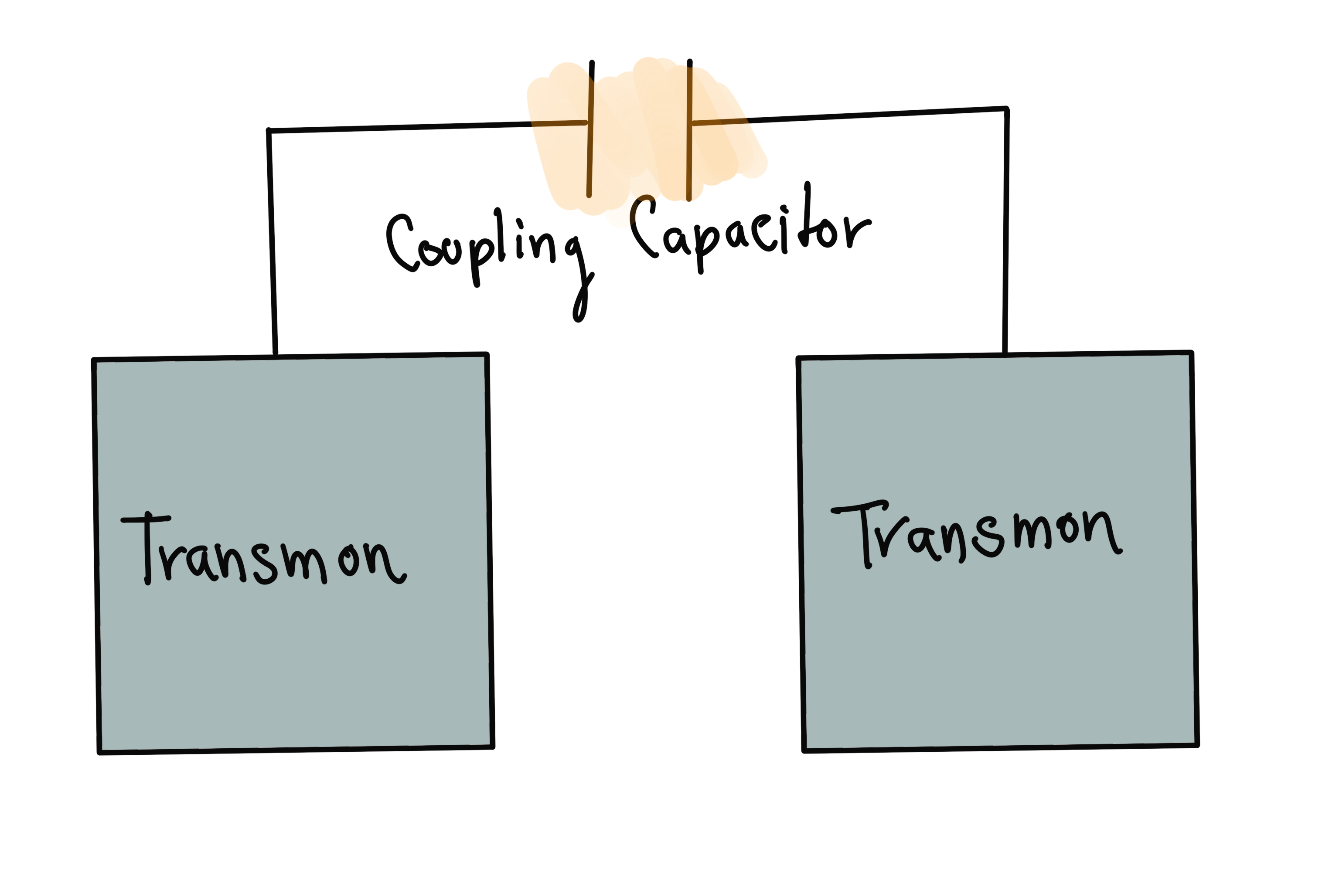
Two transmons connected through a coupling capacitor

As we will see, this capacitor helps us have a controlled interaction between qubits. When two identical transmons are connected through a coupling capacitor, the Hamiltonian for the system of two qubits reads 6

\[\hat{H}=\frac{\hbar J}{2} (\sigma^{x}_1\sigma^{x}_2+\sigma^{y}_1\sigma^{y}_2),\]

where \(J\) depends on the coupling capacitance and the characteristics of both circuits. Note that since the transmons are identical, they have the same energy gap. The Hamiltonian \(\hat{H}\) allows us to implement the two-qubit \(iSWAP\) gate

\[\begin{split}iSWAP = \left( \begin{array}{cccc} 1 & 0 & 0 & 0 \\ 0 & 0 & i & 0 \\ 0 & i & 0 & 0 \\ 0 & 0 & 0 & 1 \end{array} \right)\end{split}\]

when applied for a time \(t=3\pi/2J\), as shown with the following PennyLane code:

dev3 = qml.device("default.qubit", wires=2)

# Define Hamiltonian
coeffs = [0.5, 0.5]
ops = [qml.PauliX(0) @ qml.PauliX(1), qml.PauliY(0) @ qml.PauliY(1)]

Two_qubit_H = qml.Hamiltonian(coeffs, ops)

# Implement Hamiltonian evolution for time t and some initial computational basis state
@qml.qnode(dev3, interface="autograd")
def Sc_ISWAP(basis_state, time):
    qml.templates.BasisStatePreparation(basis_state, wires=range(2))
    ApproxTimeEvolution(Two_qubit_H, time, 1)
    return qml.state()


# Implement ISWAP exactly
@qml.qnode(dev3, interface="autograd")
def iswap(basis_state):
    qml.templates.BasisStatePreparation(basis_state, wires=range(2))
    qml.ISWAP(wires=[0, 1])
    return qml.state()


# Print to compare results

print("State |0>|0>:")
print(
    "Evolved for t=3*pi/2: {}; Output of ISWAP gate: {}\n ".format(
        Sc_ISWAP([0, 0], 3 * np.pi / 2).round(2), iswap([0, 0]).round(2)
    )
)

print("State |0>|1>:")
print(
    "Evolved for t=3*pi/2: {}; Output of ISWAP gate: {}\n ".format(
        Sc_ISWAP([0, 1], 3 * np.pi / 2).round(2), iswap([0, 1]).round(2)
    )
)

print("State |1>|0>:")
print(
    "Evolved for t=3*pi/2: {}; Output of ISWAP gate: {}\n ".format(
        Sc_ISWAP([1, 0], 3 * np.pi / 2).round(2), iswap([1, 0]).round(2)
    )
)

print("State |1>|1>:")
print(
    "Evolved for t=3*pi/2: {}; Output of ISWAP gate: {}\n ".format(
        Sc_ISWAP([1, 1], 3 * np.pi / 2).round(2), iswap([1, 1]).round(2)
    )
)

Out:

State |0>|0>:
Evolved for t=3*pi/2: [ 1.-0.j -0.-0.j -0.-0.j -0.-0.j]; Output of ISWAP gate: [1.+0.j 0.+0.j 0.+0.j 0.+0.j]

State |0>|1>:
Evolved for t=3*pi/2: [0.+0.j 0.-0.j 0.+1.j 0.+0.j]; Output of ISWAP gate: [0.+0.j 0.+0.j 0.+1.j 0.+0.j]

State |1>|0>:
Evolved for t=3*pi/2: [0.+0.j 0.+1.j 0.-0.j 0.+0.j]; Output of ISWAP gate: [0.+0.j 0.+1.j 0.+0.j 0.+0.j]

State |1>|1>:
Evolved for t=3*pi/2: [-0.+0.j -0.-0.j -0.-0.j  1.-0.j]; Output of ISWAP gate: [0.+0.j 0.+0.j 0.+0.j 1.+0.j]

To allow for universal computation, we must be able to build the CNOT gate by using only the ISWAP gate and any number of single-qubit gates. The following quantum circuit diagram depicts how we can achieve this 6.

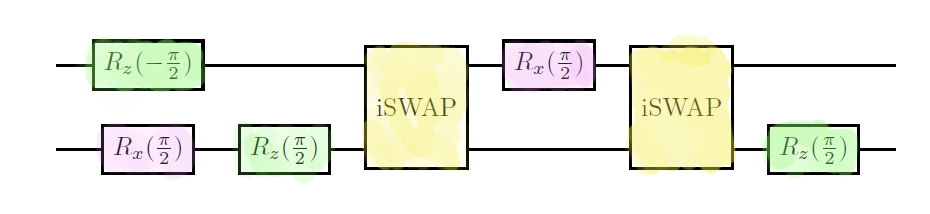
Circuit to obtain the CNOT gate from the ISWAP gate

We can verify that the circuit above gives us the CNOT gate up to a global phase using PennyLane:

def cnot_with_iswap():
    qml.RZ(-np.pi / 2, wires=0)
    qml.RX(np.pi / 2, wires=1)
    qml.RZ(np.pi / 2, wires=1)
    qml.ISWAP(wires=[0, 1])
    qml.RX(np.pi / 2, wires=0)
    qml.ISWAP(wires=[0, 1])
    qml.RZ(np.pi / 2, wires=1)


# Get matrix of circuit above
matrix = qml.matrix(cnot_with_iswap)()

# Multiply by a global phase to obtain CNOT
(np.exp(1j * np.pi / 4) * matrix).round(2)

Out:

array([[ 1.+0.j,  0.+0.j,  0.+0.j,  0.+0.j],
       [-0.+0.j,  1.-0.j,  0.+0.j,  0.+0.j],
       [ 0.+0.j,  0.+0.j, -0.+0.j,  1.+0.j],
       [ 0.+0.j,  0.+0.j,  1.-0.j,  0.+0.j]])

In the code above, we assumed that we can switch the interaction on and off to control its duration. How do we do this without physically tampering with the qubits? The truth is that we can never switch the interaction off completely, but we can weaken it greatly by changing the characteristics of one of the qubits. For example, if we change the inductance in one of the circuits to be much different from the other, the interaction strength \(J\) in the Hamiltonian will be almost zero.

This strategy, however, begs another question: how can we change the characteristics of the circuit elements on-demand? One possibility is to use flux-tunable qubits, also known as superconducting quantum interference devices (SQUIDs). They use two parallel Josephson junctions placed around each circuit, a setup that allows us to change the inductance of one qubit using an external magnetic field. This architecture, although fast, requires further interaction with the qubit, so there’s some probability of unintentionally changing its state.

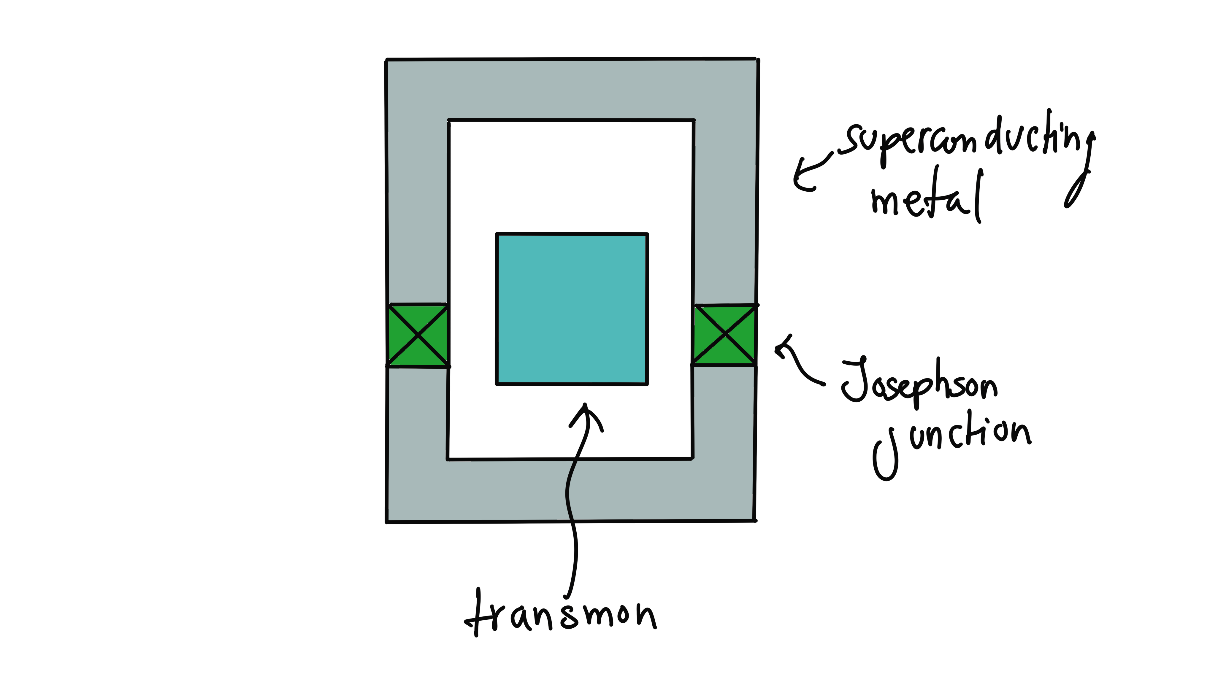
SQUID architecture surrounding a transmon

Another option is to use all-microwave gates. In this scenario, we place two different transmons in a single cavity, and shine microwaves that can be absorbed by the second qubit. The first qubit will scatter the photons, and the other will absorb them, causing a similar effect to that of the qubit-cavity system in the case of measurement. This means that we can entangle the two qubits. When the first qubit receives a microwave at the frequency that stimulates the second qubit, one can show that the (simplified) Hamiltonian is given by 7

\[\hat{H}=\hbar \tilde{\Omega} (\sigma^{z}_1\sigma^{x}_2\cos\phi+\sigma^{z}_1\sigma^{y}_2\sin\phi),\]

where \(\phi\) is the phase of the wave. As promised, we can obtain an entangled state by concatenating the evolution under this Hamiltonian for a time \(t=\tfrac{\pi}{4\Omega}\) with \(R_x\) and \(R_y\) rotations and a qml.Hadamard gate:

@qml.qnode(dev3, interface="autograd")
def H_evolve(state, phi, time):
    # Prepare initial state
    qml.templates.BasisStatePreparation(state, wires=range(2))
    # Define Hamiltonian
    coeffs = [np.cos(phi), np.sin(phi)]
    ops = [qml.PauliZ(0) @ qml.PauliX(1), qml.PauliZ(0) @ qml.PauliY(1)]
    Ham = qml.Hamiltonian(coeffs, ops)
    # Combine Hamiltonian evolution with single-qubit gates
    qml.Hadamard(wires=0)
    qml.RX(-np.pi / 2, wires=1)
    ApproxTimeEvolution(Ham, time, 1)
    qml.RZ(-np.pi / 2, wires=0)
    return qml.state()


# Verify that we return maximally entangled state up to a global phase
(np.exp(-1j * np.pi / 4) * H_evolve([0, 0], 0, np.pi / 4)).round(3)

Out:

tensor([0.707-0.j, 0.   +0.j, 0.   -0.j, 0.707+0.j], requires_grad=True)

Although this method does not affect the qubit’s state much, these gates are slower than those built using flux-tuning, since the Rabi frequency for this interaction turns out to be smaller.

Historical note: In the literature, you may find some proper names for particular types of coupled transmons. One of the most common is the xmon, which are transmons coupled with a “+” shaped capacitor. A further improvement over the xmon is the gmon, which adds an additional inductor to the coupling to better switch interactions on and off. Many more architectures have been proposed since the introduction of the xmon and the gmon, so we have reached a point where it is better to avoid getting lost in names. Understanding the basic principles introduced above will make us go a long way!

The state of the art

Superconducting qubits are a force to be reckoned with as practical implementations of quantum computers. Nonetheless, there are still some technological challenges preventing them from scaling further. A glaring issue is that we need to keep the transmons at very low temperatures, which requires the use of large cryogenic devices known as dilution refrigerators. However, many quantum computing technologies need to use cryogenic devices for different reasons. In the future, other quantum technologies may bypass the use of low temperatures, but superconducting qubits may not be so lucky, since they are constrained by the laws of physics that allow for superconductivity.

In terms of Di Vincenzo’s criteria, the long coherence times required by the third criterion have been rather hard to achieve. Superconducting circuits are large compared to other quantum systems, so their interaction with the environment is difficult to control. As a consequence, the excited state lasts for about 1 micro-second before decaying back to the ground state. Current single-qubit gates are acceptable since they can be applied in a matter of nanoseconds, thanks to our ability to manufacture very small cavities. Problems arise, however, when we want to perform precise measurements of the qubit. We’ve already seen that taking a longer time to perform a measurement gives us better precision. But there is an additional issue: the Hamiltonian we wrote in the measurement section is only valid when the number of photons in the cavity does not exceed some critical number. This upper bound on the photons sets additional constraints: we will need longer times to resolve the state, since we have few photons available to us.

Speeding up measurements without losing precision is a hot research topic in superconductor quantum computing. The primary approach has been to make the most out of the limited number of photons we have by reducing all possible environmental noise. Currently, we can perform measurements in about 50 nanoseconds with 1% error. However, since frequent measurements are needed for error correction, better precision and shorter times are required to scale our architectures further.

An additional challenge is the execution of the multi-qubit gates, which are currently ten times slower than single-qubit gates. One contender to the fastest two-qubit gate is used by Google, where the qubits are coupled with a capacitor and a SQUID. The net effect is a quick flux-tunable qubit, where the coupling \(J\) is changed by using a magnetic flux that goes through the coupling SQUID. While slower, IBM prefers to use all-microwave gates to increase coherence times. Both approaches have the problem of frequency crowding: if we interconnect too many qubits together inside a cavity, they may start to have similar energy gaps. In that case, we may manipulate qubits that we did not intend to. The problem can be somewhat addressed by changing the geometry in which the qubits are connected 8. However, much more work needs to be done to address this scalability issue.

Conclusion

Superconducting quantum computing has gained momentum in the last decade as a leading competitor in the race for building a functional quantum computer. It is based on artificial versions of atomic systems done using superconducting circuits, which allows for versatility and control. They have been easy to scale so far, but increasing the qubit coherence time and the speed of quantum operations and measurements is essential to scaling this technology further. This has motivated so many approaches for gates and measurement that we could not possibly cover them all in one demo. Do check the literature below if you’d like to learn more!

References

1

Arute, F., Arya, K., Babbush, R. et al. (2019) “Quantum supremacy using a programmable superconducting processor”, Nature 574, 505-510.

2

“IBM Unveils Breakthrough 127-Qubit Quantum Processor”. IBM Newsroom. Retrieved 2022-03-15.

3

D. DiVincenzo. (2000) “The Physical Implementation of Quantum Computation”, Fortschritte der Physik 48 (9–11): 771–783. (arXiv)

4

Bergou, J., Hillery, M., and Saffman, M. (2021) “Quantum Information Processing”, Springer.

5(1,2)

Blais, A., Grimsmo, A., Girvin, S., and Walraff, A. (2021) “Circuit quantum electrodynamics”, Rev. Mod. Phys. 93, 025005. (arXiv)

6(1,2)

Schuch, N., Siewert, J. (2003) “Natural two-qubit gate for quantum computation using the XY interaction”, Phys. Rev. A 67, 032301. (arXiv)

7

Rigetti, C., Devoret, M. (2009) “Fully microwave-tunable universal gates in superconducting qubits with linear couplings and fixed transition frequencies”, Phys. Rev. B 81, 134057.

8

“The IBM Quantum heavy hex lattice”. IBM Research Blog. Retrieved 2022-03-15

About the author

Alvaro Ballon

Alvaro is a quantum computing educator at Xanadu. His work involves making the latest developments in quantum computing accessible to the community.

demos/tutorial_sc_qubits

 

Download Python script

 

Download Notebook

 

View on GitHub