Photonic quantum computers

Author: Alvaro Ballon — Posted: 31 May 2022. Last updated: 16 June 2022.

To create a functional quantum computer, we need to produce and control a large number of qubits. This feat has proven difficult, although significant progress has been made using trapped ions, superconducting circuits, and many other technologies. Scalability—the ability to put many qubits together—is limited because individual qubits in a multi-qubit system lose their quantum properties quickly. This phenomenon, known as decoherence, happens due to the interactions of the qubits with their surroundings. One way to get scalable structures is to use photons (particles of light). The quantum states of photons are more robust against decoherence, so we may be onto something!

Indeed, many approaches to use photons for quantum computing have been proposed. We will focus on linear optical quantum computing, an approach that has already achieved quantum advantage. It is being developed further by Xanadu, PsiQuantum, and other institutions around the globe. Unlike other physical systems, photonics allows us access to an infinite number of states. How can we leverage these extra states to make quantum computers? By the end of this demo, you will be able to explain how photonic devices can be used to build universal quantum computers. You will learn how to prepare, measure, and manipulate the quantum states of light, and how we can encode qubits in photons. Moreover, you will identify the strengths and weaknesses of photonic devices in terms of Di Vincenzo’s criteria, introduced in the blue box below.

Di Vincenzo’s criteria: In the year 2000, David DiVincenzo proposed a wishlist for the experimental characteristics of a quantum computer 1. DiVincenzo’s criteria have since become the main guideline for physicists and engineers building quantum computers:

1. Well-characterized and scalable qubits. Many of the quantum systems that we find in nature are not qubits, so we must find a way to make them behave as such. Moreover, we need to put many of these systems together.

2. Qubit initialization. We must be able to prepare the same state repeatedly within an acceptable margin of error.

3. Long coherence times. Qubits will lose their quantum properties after interacting with their environment for a while. We would like them to last long enough so that we can perform quantum operations.

4. Universal set of gates. We need to perform arbitrary operations on the qubits. To do this, we require both single-qubit gates and two-qubit gates.

5. Measurement of individual qubits. To read the result of a quantum algorithm, we must accurately measure the final state of a pre-chosen set of qubits.

Our journey will start by defining the simplest states of light, known as Gaussian states. We will also describe how we can perform simple gates and measurements on such states. The next step is to figure out reliable methods to generate the more general non-Gaussian states that are required for universal quantum computing. We’ll see that we end up needing only a special type of non-Gaussian states, known as GKP states. Finally, we will bring all the concepts together to understand how quantum algorithms can be performed using these tools. Let’s get started!

Gaussian states of light

Why are the quantum states of light so durable? Photons seldom interact with each other, which means we can easily avoid uncontrolled interactions that destroy their quantum state. However, to build a universal quantum computer, we need multi-qubit gates, which means that photons must be made to communicate with each other somehow! We can make photons affect each other by using a material as a mediator. To start with, we will focus on manipulating photons using linear materials, whose properties are unchanged when they interact with light. With linear materials, we can produce a subset of the so-called Gaussian states. They can be fabricated with a 100% success rate using common optical devices, so they are our safest tool in photonics.

To precisely define a Gaussian state, we need a mathematical representation for states of light. As is the case with qubits, states of light are represented by a linear combination of basis vectors. But unlike qubits, two basis vectors aren’t enough. The reason is that light is characterized by its so-called position and momentum quadratures \(x\) and \(p,\) captured by the operators \(\hat{X}\) and \(\hat{P}\) respectively. Upon measurement, these quadratures can take any real value, which means that \(\hat{X}\) and \(\hat{P}\) have infinitely many eigenvectors. Therefore, to describe a quantum of light \(\left\lvert \psi \right\rangle,\) we need infinitely many basis vectors!

Note

The position and momentum quadratures \(x\) and \(p\) do not represent the position and momentum of one photon. They describe the state of possibly many photons, and they are related to the amplitude and phase of light. The names come from the fact that the quadrature observables \(\hat{X}\) and \(\hat{P}\) satisfy

\[\left[ \hat{X},\hat{P}\right]=i\hbar,\]

which is the same relation satisfied by conventional position and momentum in quantum mechanics. This means that no simultaneous measurement of \(\hat{X}\) and \(\hat{P}\) can be performed. Moreover, the standard deviations of the measurements of \(x\) and \(p\) satisfy the uncertainty relation

\[\Delta x \Delta p \geq 1,\]

where we work in units where \(\hbar = 2.\) Sometimes the word “quadratures” is omitted for simplicity.

For example, we write

\[\left\lvert \psi \right\rangle = \int_\mathbb{R}\psi(x)\vert x \rangle dx,\]

where \(\vert x \rangle\) is the eigenstate of \(\hat{X}\) with eigenvalue \(x,\) and \(\psi\) is a complex-valued function known as the wave function. A similar expansion can be done in terms of the eigenstates \(\vert p \rangle\) of \(\hat{P}.\) Note that an integral is used here rather than an infinite sum because the eigenvalues of \(\hat{X}\) and \(\hat{P}\) are continuous. So how do we define a Gaussian state using this representation? It is a state that is completely determined by the average values \(\bar{x}\) and \(\bar{p}\) of the position and momentum quadratures, as well as their standard deviations \(\Delta x\) and \(\Delta p.\) The most trivial Gaussian state is the vacuum—the state with no photons. Let us see what happens if we sample measurements of the quadratures \(\hat{X}\) and \(\hat{P}\) when light is in the vacuum. We can use PennyLane’s default.gaussian device, which lets us create, manipulate, and measure Gaussian states of light. Let’s first call the usual imports,

import pennylane as qml
from pennylane import numpy as np
import matplotlib.pyplot as plt

and define the device.

dev = qml.device("default.gaussian", wires=1, shots=1000)

Important

What do the wires represent in a photonic device? They are independent information carriers known as qumodes. In photonic quantum computers, these are waves of light contained inside an optical cavity. Qumodes are not two-level systems in general, so we must use an infinite superposition of basis states to represent their quantum state.

We would like to know how the measured values of position and momentum are distributed in the \(x\)-\(p\) space, usually called phase space. The initial state in default.gaussian is the vacuum, so the circuits to measure the quadratures need not contain any operations, except for measurements! We plot 1000 measurement results for both \(x\) and \(p.\)

@qml.qnode(dev)
def vacuum_measure_x():
    return qml.sample(qml.X(0))  # Samples X quadratures


@qml.qnode(dev)
def vacuum_measure_p():
    return qml.sample(qml.P(0))  # Samples P quadrature


# Sample measurements in phase space
x_sample = vacuum_measure_x()
p_sample = vacuum_measure_p()

# Import some libraries for a nicer plot
from scipy.stats import gaussian_kde
from numpy import vstack as vstack

# Point density calculation
xp = vstack([x_sample, p_sample])
z = gaussian_kde(xp)(xp)

# Sort the points by density
sorted = z.argsort()
x, y, z = x_sample[sorted], p_sample[sorted], z[sorted]

# Plot
fig, ax = plt.subplots()
ax.scatter(x, y, c = z, s = 50, cmap="RdYlGn")
plt.title("Vacuum", fontsize=12)
ax.set_ylabel("Momentum", fontsize = 11)
ax.set_xlabel("Position", fontsize = 11)
ax.set_aspect("equal", adjustable = "box")
plt.show()

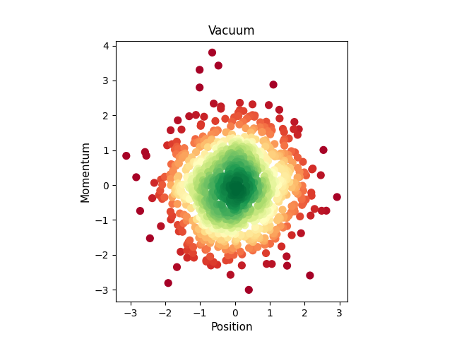
We observe that the values of the quadratures are distributed around the origin with a spread of approximately 1. We can check these eyeballed values explicitly, using a device without shots this time.

dev_exact = qml.device("default.gaussian", wires=1)  # No explicit shots gives analytic calculations


@qml.qnode(dev_exact)
def vacuum_mean_x():
    return qml.expval(qml.X(0))  # Returns exact expecation value of x


@qml.qnode(dev_exact)
def vacuum_mean_p():
    return qml.expval(qml.P(0))  # Returns exact expectation value of p


@qml.qnode(dev_exact)
def vacuum_var_x():
    return qml.var(qml.X(0))  # Returns exact variance of x


@qml.qnode(dev_exact)
def vacuum_var_p():
    return qml.var(qml.P(0))  # Returns exact variance of p


# Print calculated statistical quantities
print("Expectation value of x-quadrature: {}".format(vacuum_mean_x()))
print("Expectation value of p-quadrature: {}".format(vacuum_mean_p()))
print("Variance of x-quadrature: {}".format(vacuum_var_x()))
print("Variance of p-quadrature: {}".format(vacuum_var_p()))

Out:

Expectation value of x-quadrature: 0.0
Expectation value of p-quadrature: 0.0
Variance of x-quadrature: 1.0
Variance of p-quadrature: 1.0

But where does the name Gaussian come from? If we plot the density of quadrature measurements for the vacuum state in three dimensions, we obtain the following plot.

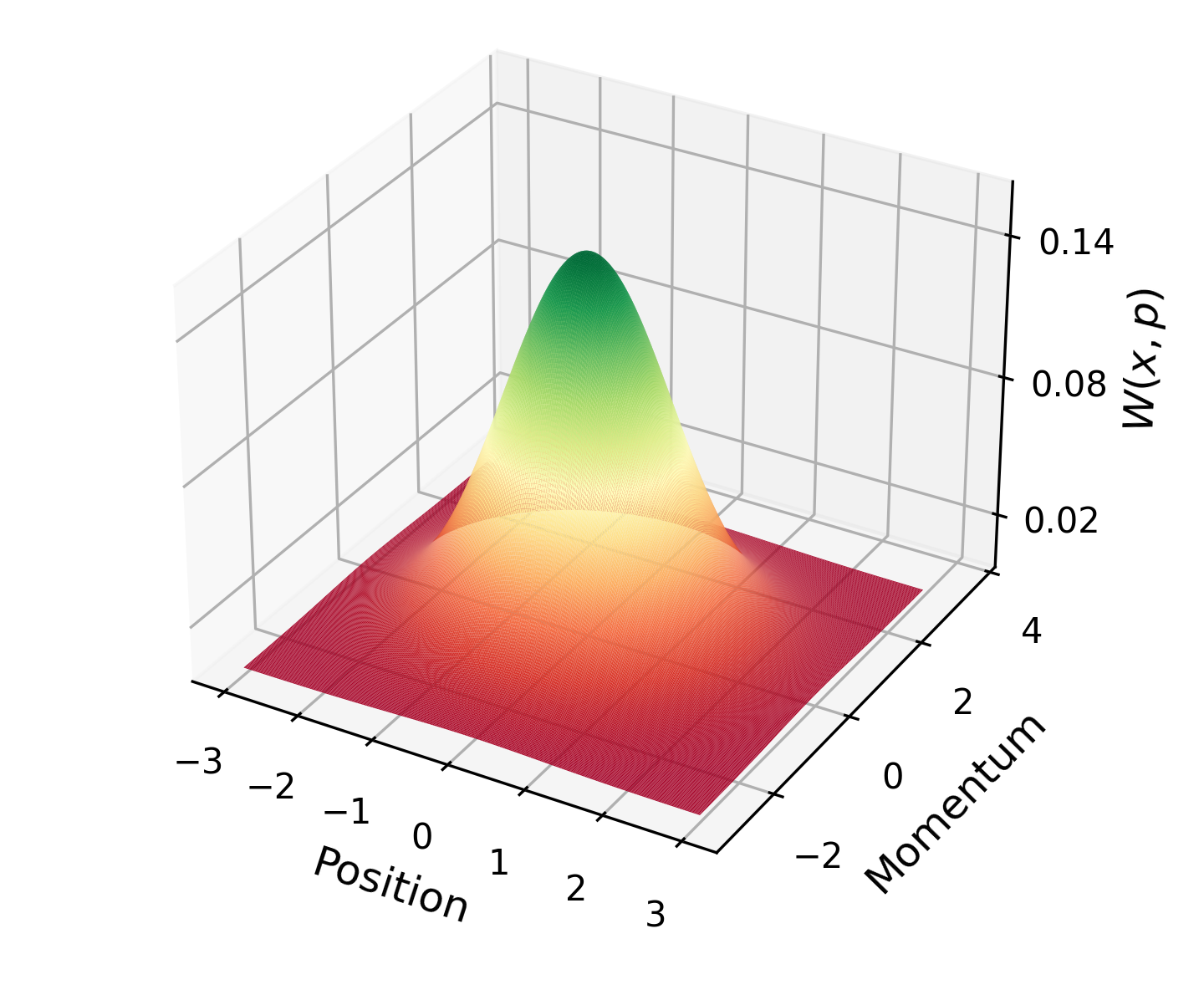
Density of measurement results in phase space for the vacuum state

The density has the shape of a 2-dimensional Gaussian surface, hence the name. For Gaussian states only, the density is exactly equal to the so-called Wigner function \(W(x,p),\) defined using the wave function \(\psi(x)\):

\[W(x,p) = \frac{1}{\pi\hbar}\int_{-\infty}^{\infty}\psi^{*}(x+y)\psi(x-y)e^{2ipy/\hbar}dy.\]

Since the Wigner function satisfies

\[\int_{\mathbb{R}^2}W(x,p)dxdp = 1\]

and is positive for Gaussian states, it is almost as if the values of the momentum and position had an underlying classical probability distribution, save for the fact that the quadratures can’t be measured simultaneously. For this reason, Gaussian states are considered to be “classical” states of light. Now we’re ready for the technical definition of a Gaussian state.

Definition

A photonic system is said to be in a Gaussian state if its Wigner function is a two-dimensional Gaussian function 2.

What other Gaussian states are there? The states produced by lasers are called coherent states, which are also Gaussian with \(\Delta x = \Delta p = 1.\) Coherent states, in general, can have non-zero expectation values for the quadratures (i.e., they are not centered around the origin).

The default.gaussian device allows for the easy preparation of coherent states through the function CoherentState, which takes two parameters \(\alpha\) and \(\phi.\) Here, \(\alpha=\sqrt{\vert\bar{x}\vert^2+\vert\bar{p}\vert^2}\) is the magnitude and \(\phi\) is the polar angle of the point \((\bar{x}, \bar{p}).\) Let us plot sample quadrature measurements for a coherent state.

@qml.qnode(dev)
def measure_coherent_x(alpha, phi):
    qml.CoherentState(alpha, phi, wires=0)  # Prepares coherent state
    return qml.sample(qml.X(0))  # Measures X quadrature


@qml.qnode(dev)
def measure_coherent_p(alpha, phi):
    qml.CoherentState(alpha, phi, wires=0)  # Prepares coherent state
    return qml.sample(qml.P(0))  # Measures P quadrature


# Choose alpha and phi and sample 1000 measurements
x_sample_coherent = measure_coherent_x(3, np.pi / 3)
p_sample_coherent = measure_coherent_p(3, np.pi / 3)

# Plot as before
xp = vstack([x_sample_coherent, p_sample_coherent])
z1 = gaussian_kde(xp)(xp)

sorted = z1.argsort()
x, y, z = x_sample_coherent[sorted], p_sample_coherent[sorted], z1[sorted]

fig, ax1 = plt.subplots()
ax1.scatter(x, y, c = z, s = 50, cmap = "RdYlGn")
ax1.set_title("Coherent State", fontsize = 12)
ax1.set_ylabel("Momentum", fontsize = 11)
ax1.set_xlabel("Position", fontsize = 11)
ax1.set_aspect("equal", adjustable = "box")
plt.xlim([-0.5, 8])
plt.ylim([0, 9])
plt.show()

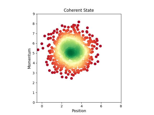
Indeed, we see that the distribution of quadrature measurements is similar to that of the vacuum, except that it is not centered at the origin. Instead it is centred at the alpha and phi coordinates we chose in the code above.

Gaussian operations

We have only learned about two types of Gaussian states so far. The vacuum can be obtained by carefully isolating a system from any environmental influences, and a coherent state can be produced by a laser, so we already have these at hand. But how can we obtain any Gaussian state of our liking? This is achieved through Gaussian operations, which transform a Gaussian state to another Gaussian state. These operations are relatively easy to implement in a lab using some of the optical elements introduced in the table below.

Element	Diagram	Description
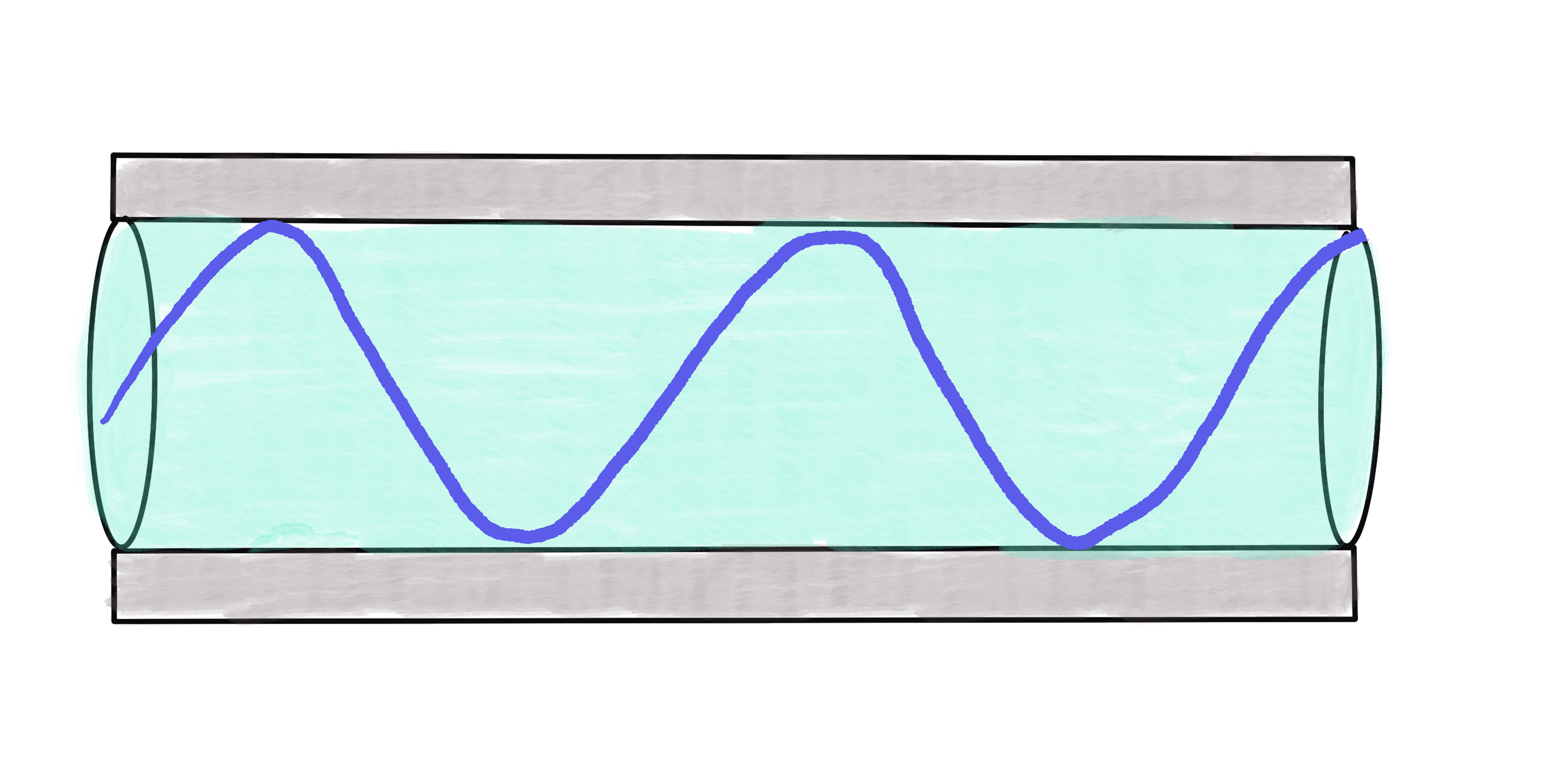
Waveguide		A long strip of material that contains and guides electromagentic waves. For example, an optical fibre is a type of waveguide.
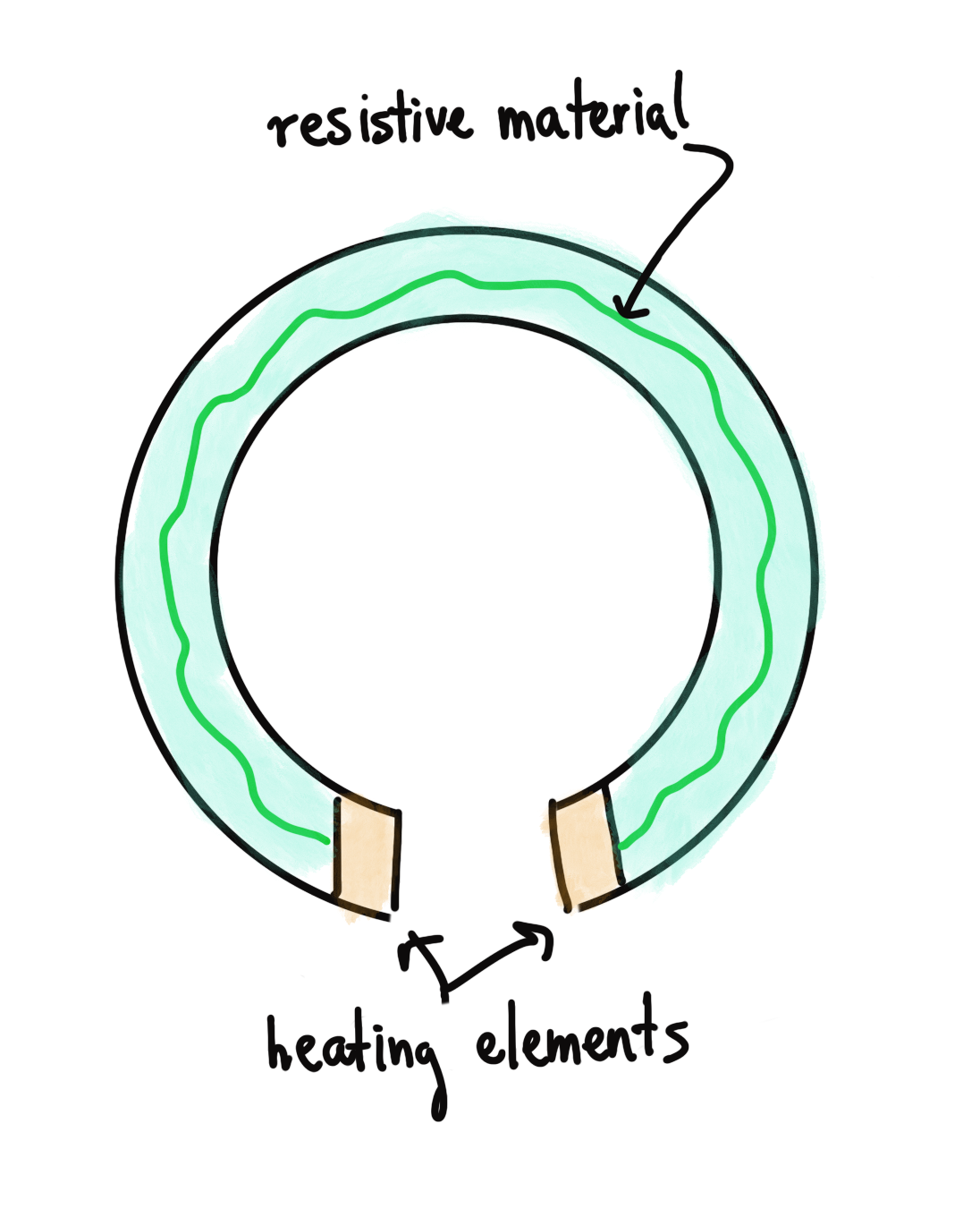
Phase-shifter		A piece of material that changes the phase of light. The figure shows a particular implementation known as a thermo-optic phase shifter 3, which is a (sometimes curved) waveguide that changes properties when heated up using a resistor. This allows us to control the applied phase difference.
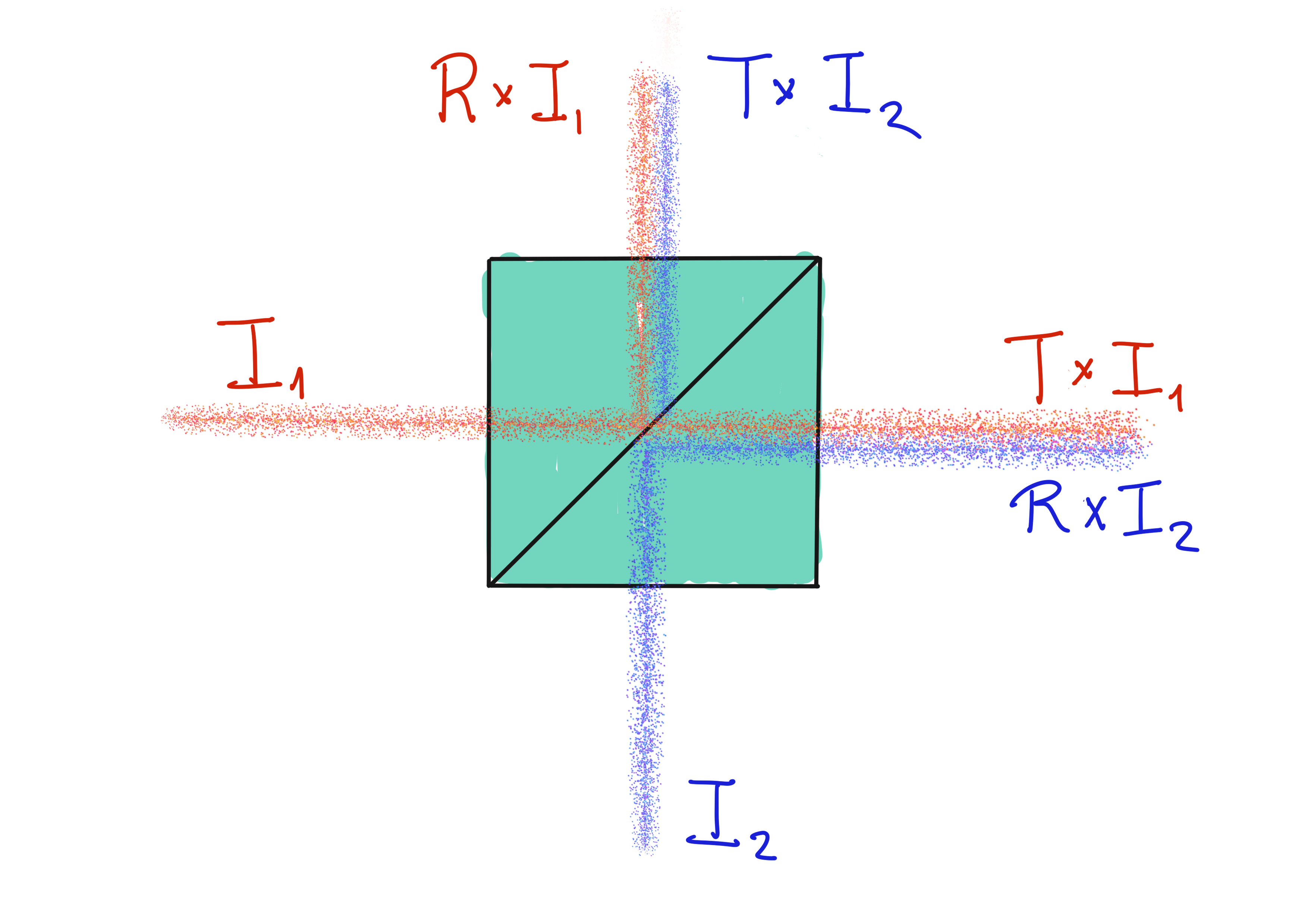
Beamsplitter		An element with two input and two output qumodes. It transmits a fraction \(T\) of the photons coming in through either entry port, and reflects a fraction \(R=1-T.\) The input qumodes can be combined to create entangled states across the output ports. In a photonic quantum computing chip, a directional coupler is used.

The vacuum is centered at the origin in phase space. It is advantageous to generate states that are centered at any point in phase space. How would we, for example, change the mean \(\bar{x}\) of the \(x\)-quadrature without changing anything else about the state? This can be done via the displacement operator, implemented in PennyLane via Displacement. Let’s see the effect of this operation on an intial coherent state.

@qml.qnode(dev)
def displace_coherent_x(alpha, phi, x):
    qml.CoherentState(alpha, phi, wires = 0)  # Create coherent state
    qml.Displacement(x, 0, wires = 0)  # Second argument is the displacement direction in phase space
    return qml.sample(qml.X(0))


@qml.qnode(dev)
def displace_coherent_p(alpha, phi, x):
    qml.CoherentState(alpha, phi, wires = 0)
    qml.Displacement(x, 0, wires = 0)
    return qml.sample(qml.P(0))


# We plot both the initial and displaced state
initial_x = displace_coherent_x(3, np.pi / 3, 0)  # initial state amounts to 0 displacement
initial_p = displace_coherent_p(3, np.pi / 3, 0)
displaced_x = displace_coherent_x(3, np.pi / 3, 3)  # displace x=3 in x-direction
displaced_p = displace_coherent_p(3, np.pi / 3, 3)
# Plot as before
fig, ax1 = plt.subplots(figsize=(10, 5))
xp1 = vstack([initial_x, initial_p])
z1 = gaussian_kde(xp1)(xp1)
sorted1 = z1.argsort()
x1, y1, z1 = initial_x[sorted1], initial_p[sorted1], z1[sorted1]
xp2 = vstack([displaced_x, displaced_p])
z2 = gaussian_kde(xp2)(xp2)
sorted2 = z2.argsort()
x2, y2, z2 = displaced_x[sorted2], displaced_p[sorted2], z2[sorted2]
ax1.scatter(x1, y1, c = z1, s = 50, cmap  ="RdYlGn")
ax1.scatter(x2, y2, c = z2, s = 50, cmap = "RdYlGn")
plt.xlim([0, 12])
plt.ylim([0, 9])
ax1.set_aspect("equal", adjustable="box")
plt.text(1, 0.8, "Before displacement")
plt.text(7.5, 0.8, "After displacement")
ax1.set_ylabel("Momentum", fontsize=11)
ax1.set_xlabel("Position", fontsize=11)
ax1.set_title("Displacing coherent states", fontsize=12)
ax1.set_aspect("equal", adjustable = "box")
plt.show()

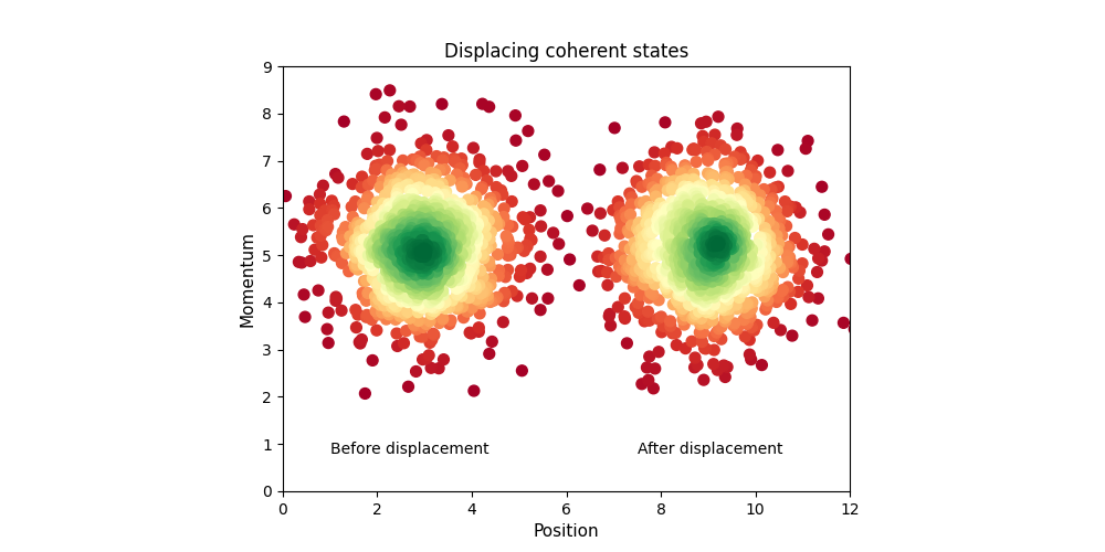
Note that setting \(x=3\) gave a displacement of 6 units in the horizontal direction in phase space. This is because the scale of phase space is set by our choice of units \(\hbar=2.\)

So how do we make a displacement operation in the lab? One method is shown below, which uses a beamsplitter and a source of high-intensity coherent light 4.

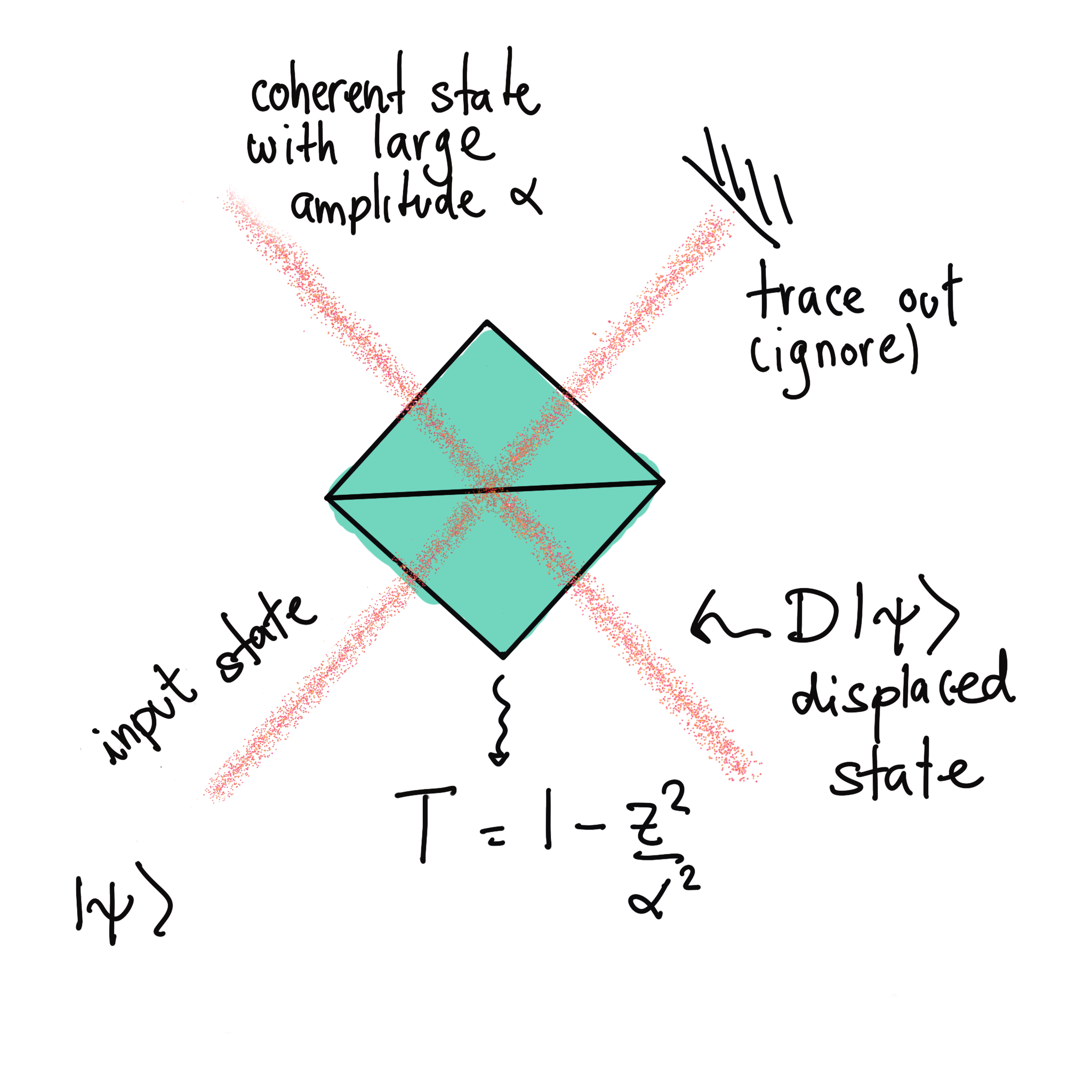
This setup displaces the input state \(\lvert\psi\rangle\) by a quantity proportional to \(z.\)

We can check that this setup implements a displacement operator using PennyLane. This time, we need two qumodes, since we rely on combining the input state that we want to displace with a coherent state in a beamsplitter. Let us code this circuit in the case that the input is a coherent state as a particular case (the operation will work for any state). Let us be mindful that this will only work when the amplitude of the input state is much smaller than that of the auxiliary coherent state.

dev2 = qml.device("default.gaussian", wires=2, shots=1000)


@qml.qnode(dev2)
def disp_optics(z, x):
    qml.CoherentState(z, 0, wires = 0)  # High-amplitude auxiliary coherent state
    qml.CoherentState(3, np.pi / 3, wires = 1)  # Input state (e.g. low amplitude coherent state)
    qml.Beamsplitter(np.arccos(1 - x ** 2 / z ** 2), 0, wires=[0, 1])  # Beamsplitter
    return qml.sample(qml.X(1))  # Measure x quadrature


@qml.qnode(dev2)
def mom_optics(z, x):
    qml.CoherentState(z, 0, wires = 0)
    qml.CoherentState(3, np.pi / 3, wires = 1)
    qml.Beamsplitter(np.arccos(1 - x ** 2 / z ** 2), 0, wires = [0, 1])
    return qml.sample(qml.P(1))  # Measure p quadrature


# Plot quadrature measurement before and after implementation of displacement
initial_x = disp_optics(100, 0)  # Initial corresponds to beamsplitter with t=0 (x=0)
initial_p = mom_optics(100, 0)  # Amplitude of coherent state must be large
displaced_x = disp_optics(100, 3)
displaced_p = mom_optics(100, 3)  # Set some non-trivial t
# Plot as before
fig, ax1 = plt.subplots()
xp1 = vstack([initial_x, initial_p])
z1 = gaussian_kde(xp1)(xp1)
sorted1 = z1.argsort()
x1, y1, z1 = initial_x[sorted1], initial_p[sorted1], z1[sorted1]
xp2 = vstack([displaced_x, displaced_p])
z2 = gaussian_kde(xp2)(xp2)
sorted2 = z2.argsort()
x2, y2, z2 = displaced_x[sorted2], displaced_p[sorted2], z2[sorted2]
ax1.scatter(x1, y1, c = z1, s = 50, cmap = "RdYlGn")
ax1.scatter(x2, y2, c = z2, s = 50, cmap = "RdYlGn")
ax1.set_title("Initial", fontsize = 12)
plt.xlim([-0.5, 15])
plt.ylim([0, 9])
ax1.set_ylabel("Momentum", fontsize = 11)
ax1.set_xlabel("Position", fontsize = 11)
plt.text(1, 0.5, "Before displacement")
plt.text(9.5, 0.5, "After displacement")
ax1.set_aspect("equal", adjustable="box")
ax1.set_title("Implementation of displacement operator", fontsize = 12)
plt.show()

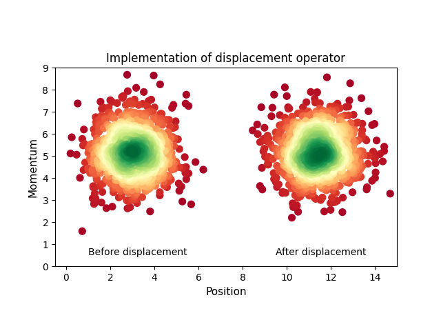
We see that we get a displaced state. The amount of displacement can be adjusted by changing the parameters of the beamsplitter. Similarly, we can implement rotations in phase space using Rotation, which simply amounts to changing the phase of light using a phase shifter. In phase space, this amounts to rotating the point \((\bar{x},\bar{p})\) around the origin.

So far, we have focused on changing the mean values of \(x\) and \(p.\) But what if we also want to change the spread of the quadratures while keeping \(\Delta x\Delta p =1\)?. This would “squeeze” the Wigner function in one direction. Aptly, the resulting state is known as a squeezed state, which is more difficult to obtain. It requires shining light through non-linear materials, where the state of light will undergo unitary evolution in a way that changes \(\Delta x\) and \(\Delta p.\)

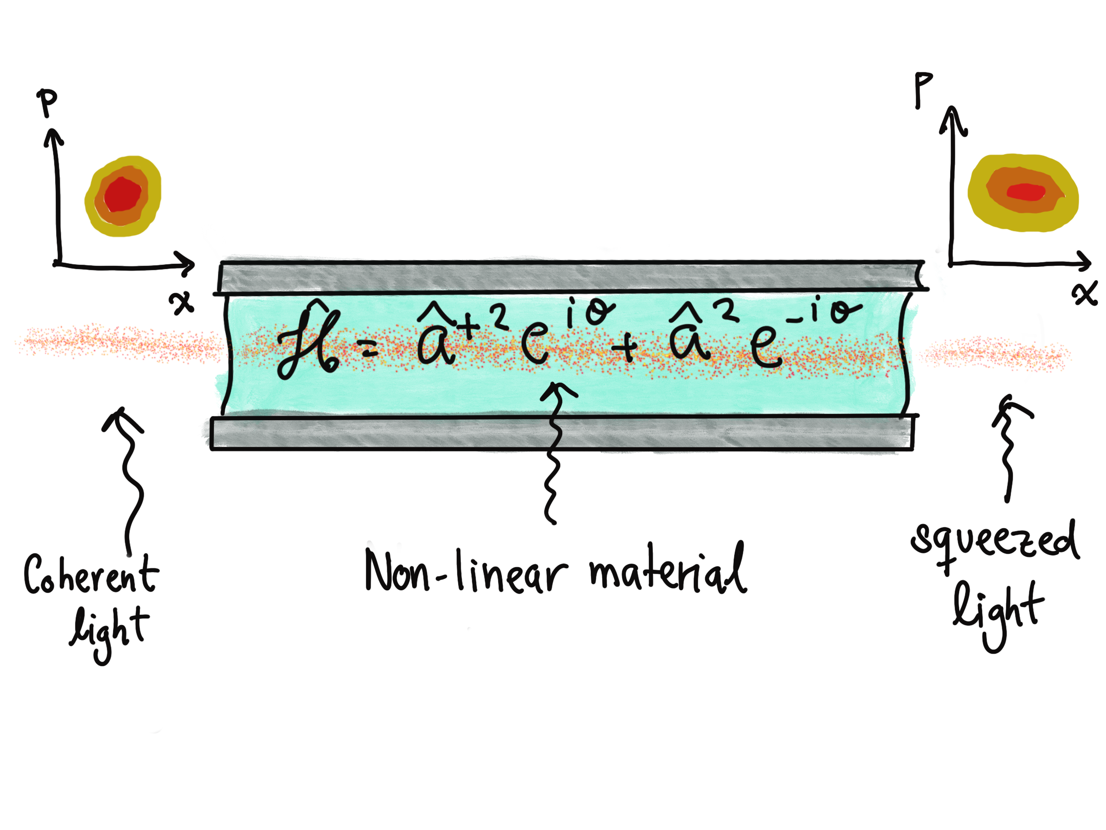
A non-linear material can work as a squeezer 5.

We won’t go into detail here, but we note that the technology to produce these states is quite mature. In PennyLane, we can generate squeezed states through the squeezing operator Squeezing. This function depends on the squeezing parameter \(r\) which tells us how much the variance in \(x\) and \(p\) changes, and \(\phi,\) which rotates the state in phase space. Let’s take a look at how squeezing changes the distribution of quadrature measurements.

@qml.qnode(dev)
def measure_squeezed_x(r):
    qml.Squeezing(r, 0, wires = 0)
    return qml.sample(qml.X(0))


@qml.qnode(dev)
def measure_squeezed_p(r):
    qml.Squeezing(r, 0, wires = 0)
    return qml.sample(qml.P(0))


# Choose alpha and phi and sample 1000 measurements
x_sample_squeezed = measure_squeezed_x(0.4)
p_sample_squeezed = measure_squeezed_p(0.4)

# Plot as before
xp = vstack([x_sample_squeezed, p_sample_squeezed])
z = gaussian_kde(xp)(xp)

sorted_meas = z.argsort()
x, y, z = x_sample_squeezed[sorted_meas], p_sample_squeezed[sorted_meas], z[sorted_meas]

fig, ax1 = plt.subplots(figsize=(7, 7))
ax1.scatter(x, y, c = z, s = 50, cmap = "RdYlGn")
ax1.set_title("Squeezed State", fontsize = 12)
ax1.set_ylabel("Momentum", fontsize = 11)
ax1.set_xlabel("Position", fontsize = 11)
ax1.set_xlim([-4, 4])
ax1.set_aspect("equal", adjustable = "box")
plt.show()

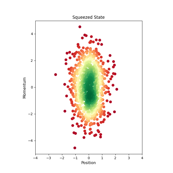
This confirms that squeezing changes the variances of the quadratures.

Note

The squeezed states produced above satisfy \(\Delta x \Delta p = 1,\) but more general Gaussian states need not satisfy these. For the purposes of photonic quantum computing, we won’t need these generalized states.

Measuring quadratures

Now that we know how to manipulate Gaussian states, we would like to perform measurements on them. So far, we have taken for granted that we can measure the quadratures \(\hat{X}\) and \(\hat{P}.\) But how do we actually measure them using optical elements? We will need a measuring device known as a photodetector. These contain a piece of a photoelectric material, where each outer electron can be stimulated by a photon. The more photons that are incident on the photodetector, the more electrons that are freed in the material, which in turn form an electric current. Mathematically,

\[I = qN,\]

where \(I\) is the electric current, \(N\) is the number of photons, and \(q\) is a detector-dependent proportionality constant 5. Hence, measuring the current amounts to measuring the number of photons indirectly!

The number of photons in a quantum of light is not fixed. It is measured by the quantum photon-number observable \(\hat{N},\) which has eigenstates denoted \(\vert 0 \rangle, \vert 1\rangle, \vert 2 \rangle,\dots\) These states, known as Fock states, do have a well-defined number of photons: repeated measurements of \(\hat{N}\) on the same state will yield the same output. The natural number \(n\) in the Fock state \(\vert n \rangle\) denotes the only possible result we would get upon measuring the photon number. But nothing prevents light from being in a superposition of Fock states. For example, when we measure \(\hat{N}\) for the state

\[\vert \psi \rangle = \frac{1}{\sqrt{3}}\left(\vert 0 \rangle + \vert 1 \rangle + \vert 2 \rangle\right),\]

we get 0, 1, or 2 photons, each with probability \(\frac{1}{3}.\)

Except for the vacuum \(\vert 0 \rangle,\) Fock states are not Gaussian. But all states of light are superpositions of Fock States, including Gaussian states! For example, let’s measure the expected photon number for some squeezed state:

dev3 = qml.device("default.gaussian", wires=1)


@qml.qnode(dev3)
def measure_n_coherent(alpha, phi):
    qml.Squeezing(alpha, phi, wires = 0)
    return qml.expval(qml.NumberOperator(0))


coherent_expval = measure_n_coherent(1, np.pi / 3)
print("Expected number of photons: {}".format(coherent_expval))

Out:

Expected number of photons: 1.3810978455418157

Since the expectation value is not an integer number, the measurement results cannot have been all the same integer. This squeezed state cannot be a Fock state!

But what about the promised quadrature measurements? We can perform them through a combination of photodetectors and a beamsplitter, as shown in the diagram below 5.

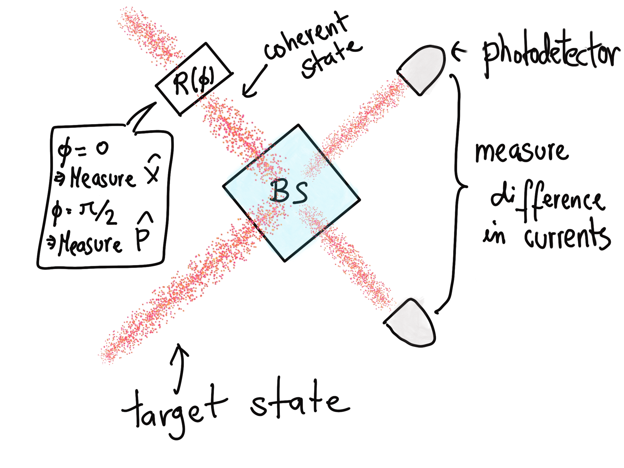
Measuring quadratures using photodetectors

Let’s code this setup using PennyLane and check that it amounts to the measurement of quadratures.

dev_exact2 = qml.device("default.gaussian", wires = 2)


@qml.qnode(dev_exact2)
def measurement(a, phi):
    qml.Displacement(a, phi, wires = 0)  # Implement displacement using PennyLane
    return qml.expval(qml.X(0))


@qml.qnode(dev_exact2)
def measurement2_0(a, theta, alpha, phi):
    qml.Displacement(a, theta, wires = 0)  # We choose the initial to be a displaced vacuum
    qml.CoherentState(alpha, phi, wires = 1)  # Prepare coherent as second qumode
    qml.Beamsplitter(np.pi / 4, 0, wires=[0, 1])  # Interfere both states
    return qml.expval(qml.NumberOperator(0))  # Read out N

@qml.qnode(dev_exact2)
def measurement2_1(a, theta, alpha, phi):
    qml.Displacement(a, theta, wires = 0)  # We choose the initial to be a displaced vacuum
    qml.CoherentState(alpha, phi, wires = 1)  # Prepare coherent as second qumode
    qml.Beamsplitter(np.pi / 4, 0, wires=[0, 1])  # Interfere both states
    return qml.expval(qml.NumberOperator(1))  # Read out N


print(
    "Expectation value of x-quadrature after displacement: {}\n".format(measurement(3, 0))
)
print("Expected current in each detector:")
print("Detector 1: {}".format(measurement2_0(3, 0, 1, 0)))
print("Detector 2: {}".format(measurement2_1(3, 0, 1, 0)))
print(
    "Difference between currents: {}".format(
        measurement2_1(3, 0, 1, 0) - measurement2_0(3, 0, 1, 0)
    )
)

Out:

Expectation value of x-quadrature after displacement: 6.0

Expected current in each detector:
Detector 1: 2.000000000000001
Detector 2: 7.999999999999998
Difference between currents: 5.999999999999997

Here we used \(q=1\) as the detector constant, but we should note that this quantity can’t really be measured precisely. However, we only care about distinguishing different states of light, so knowing the constant isn’t really needed!

Trying the above with many input states should convince you that this setup, known as homodyne measurement, allows us to measure the quadratures \(\hat{X}\) and \(\hat{P}.\) Feel free to play around changing the values of \(\phi\) and \(a\)!

Beyond Gaussian states

We’ve learned a lot about Gaussian states now, but they don’t seem to have many quantum properties. They are described by their positive Wigner function, which is to an extent analogous to a probability distribution. Are they really different from classical states? Not that much! To build a universal photonic quantum computer we need both Gaussian and non-Gaussian states. Moreover, we need to be able to entangle any two states.

Entanglement is not a problem, since combinations of Gaussian operations involving squeezers and beamsplitters can easily create entangled states! Let us set on the more challenging mission to find a way to prepare non-Gaussian states. All of the operations that we have learned so far—displacements, rotations, squeezing—are Gaussian. Do we need some kind of strange material that will implement a non-Gaussian operation? That’s certainly a possibility, and there are materials which can provide non-Gaussian interactions—like the Kerr effect. But relying on these non-linear materials is far from optimal, since the Kerr effect is weak and we don’t have much freedom to manipulate the setup into getting an arbitrary non-Gaussian state.

But there’s one non-Gausian operation that’s been right in front of our eyes all this time. The measurement of the number of photons takes a Gaussian state and collapses it into a Fock state (although this destroys the photons); therefore, photon-number detection is not a Gaussian operation. Measuring the exact number of photons is not that easy. We need fancy devices known a photon-number resolving detectors (commonly abbreviated as PNRs), which are superconductor-based, so they work only at low temperatures. Combined with squeezed states and beamsplitters, we have all the ingredients to produce non-Gaussian states.

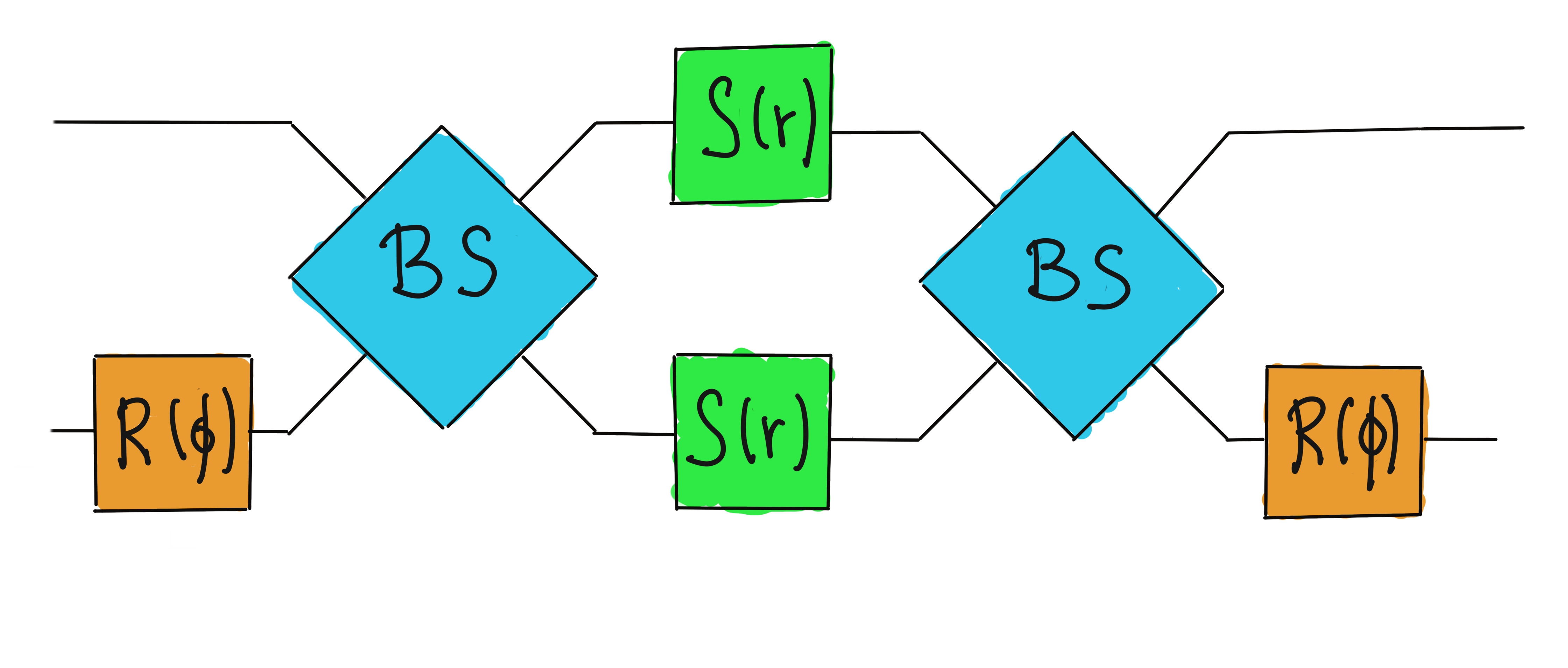
Let’s explore how this works. The main idea is to tweak a particular photonic circuit known as a Gaussian Boson Sampler 6, which is shown below.

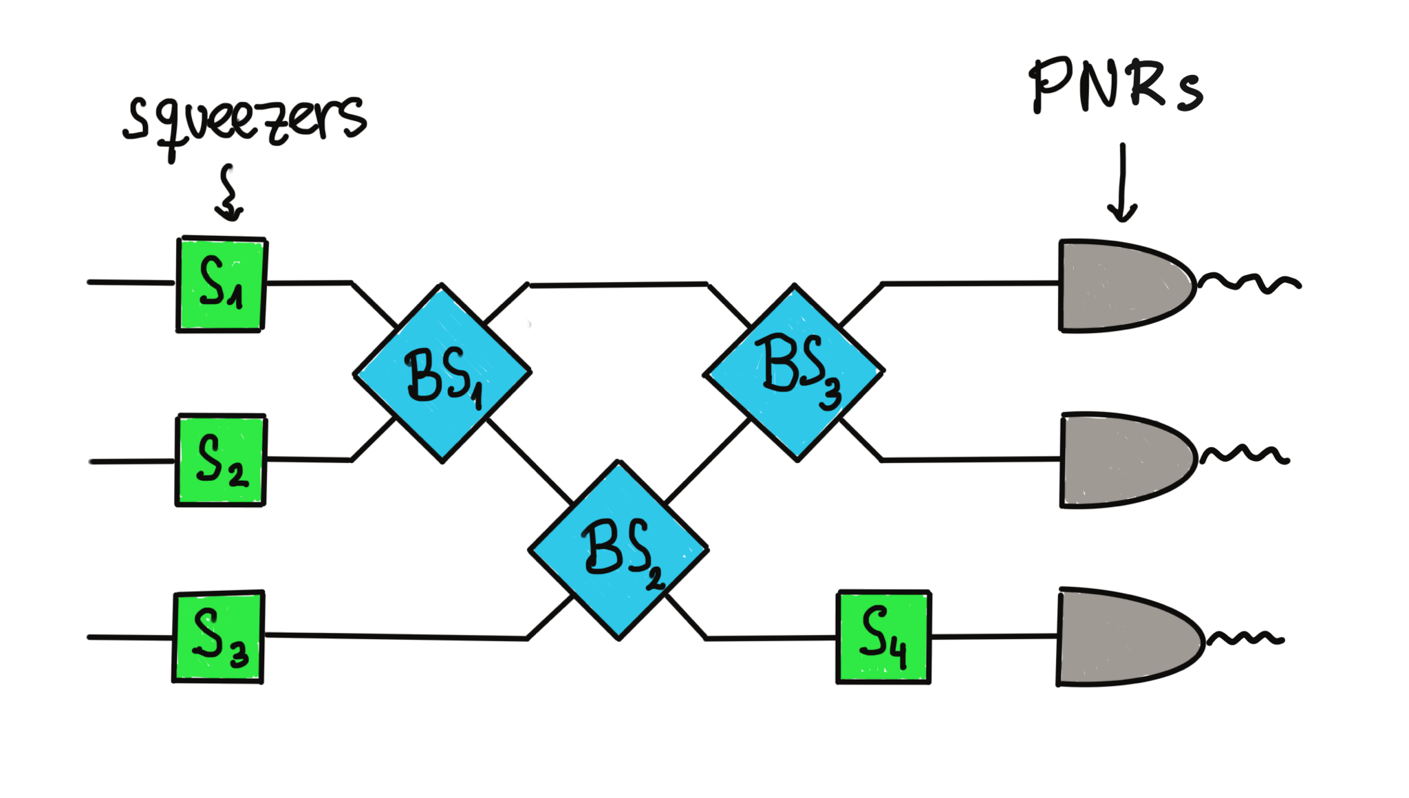
A Gaussian Boson Sampling circuit. The beamsplitters here may include phase shifts.

Gaussian boson sampling (GBS) is interesting on its own (see this tutorial for an in-depth discussion). So far, two quantum devices have used large-scale versions of this circuit to achieve quantum advantage on a particular computation, which involves sampling from a probability distribution that classical computers take too long to simulate. In 2019, USTC’s Jiuzhang device took 200 seconds to perform this sampling, which would take 2.5 billion years for some of our most powerful supercomputers 7. In 2022, Xanadu’s Borealis performed the same calculation in 36 microseconds, with the added benefit of being programmable and available on the Cloud 8.

But the most interesting application of GBS comes from removing the PNR in the last wire, as shown below.

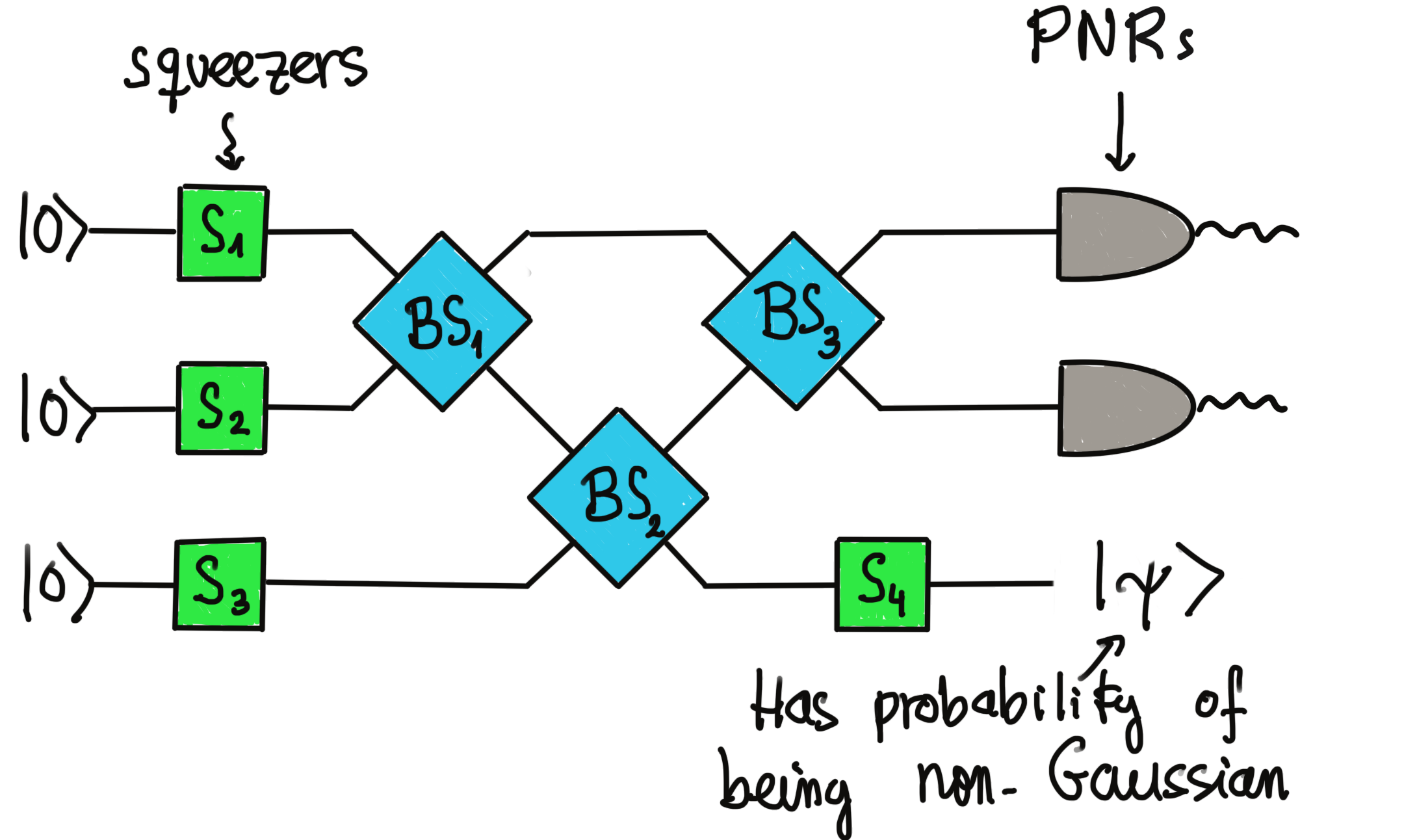
Circuit to produce non-Gaussian states probabilistically

Circuits like the above can, after photon detection of the other qumodes, produce non-Gaussian states. The reason is that the final state of the circuit is entangled, and we apply a non-Gaussian operation to some of the qumodes. This measurement affects the remaining qumode, whose state becomes non-Gaussian in general. This is the magic of quantum mechanics: due to entanglement, a measurement on a physical system can affect the state of another! Moreover, one can show that generalizations of the GBS circuit above can be built to produce any non-Gaussian state that we want 9.

For example, the choice of parameters

\[t_1 = 0.8624, \quad t_2=0.7688, \quad t_3 = 0.7848,\]

\[S_1 = -1.38, \quad S_2 = -1.22, \quad S_3 = 0.780 \quad S_4 = 0.196,\]

for this generalized GBS circuit produces, with some probability, the following state (expressed as a combination of Fock states)

\[\vert \psi \rangle = S(0.196)\left(0.661 \vert 0\rangle -0.343 \vert 2\rangle + 0.253\vert 4\rangle -0.368\vert 6\rangle +0.377 \vert 8\rangle + 0.323 \vert 10\rangle + 0.325\vert 12\rangle\right),\]

where \(S\) is the squeezing operator 9. This state’s Wigner function is shown below.

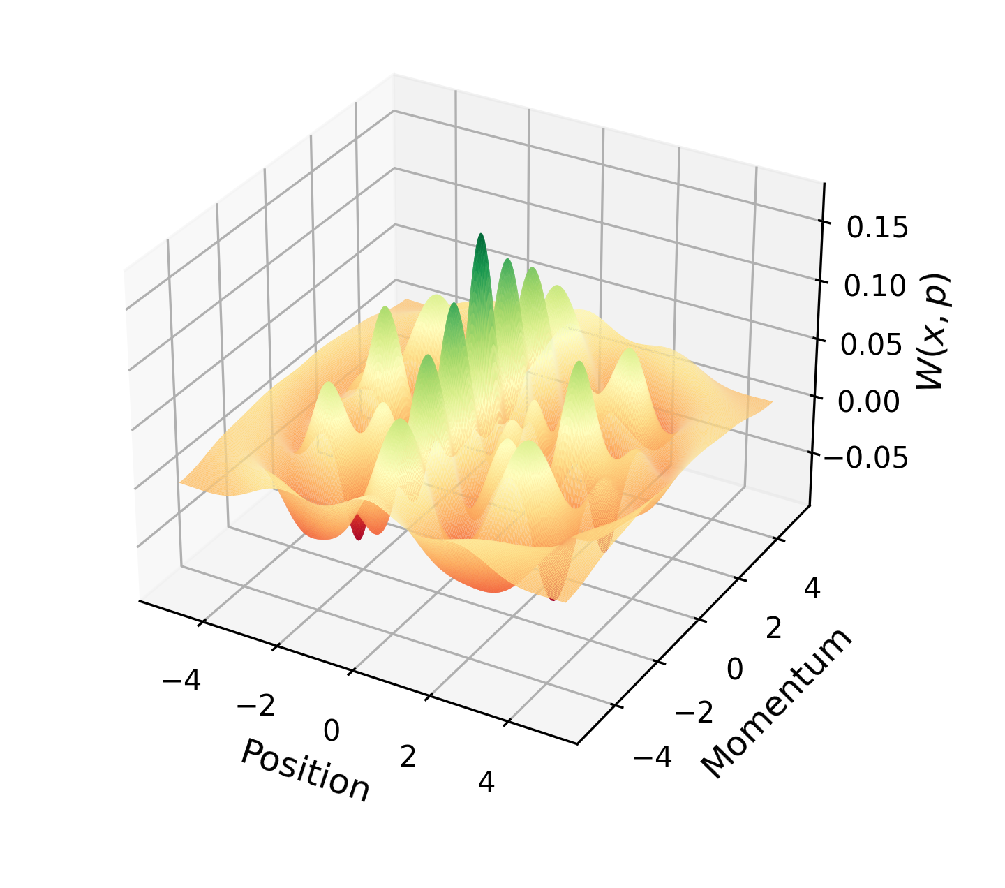
Wigner function of non-Gaussian state

This Wigner function does not have the shape of a Gaussian and moreover, it can be negative—a tell-tale feature of non-Gaussian states (we can only interpret the Wigner function as some sort of probability distribution for the case of Gaussian states!). The only issue is that the non-Gaussian state is produced only with some probability, that is, when the detectors measure some particular number of photons. But, at the very least, we can be sure that we have obtained the non-Gaussian state we wanted, and otherwise we just discard the qumode. For more precise calculations, you can check out this tutorial from PennyLane’s sister library The Walrus, which is optimized for simulating this type of circuit.

Encoding qubits into qumodes

It’s great that we can manipulate quantum states of light so freely, but we haven’t discussed how to use them for quantum computing. We would like a way to encode qubits into qumodes, so that we can run any qubit-based quantum algorithm using qumodes. Surely there’s more than one way to encode a two-dimensional subspace into an infinite-dimensional one. The only problem is that most of these encodings are extremely sensitive to the noise affecting the larger space. A way that has proven to be quite robust to errors is to encode qubits in states of light is using a special type of non-Gaussian states called GKP states 10.

GKP states are linear combinations of the following two basis states:

\[\vert 0 \rangle_{GKP} = \sum_{n} \vert 2n\pi\rangle_x,\]

\[\vert 1 \rangle_{GKP} = \sum_{n} \vert (2n+1)\pi\rangle_x,\]

where the subscript \(x\) means that the kets in the sum are eigenstates of the quadrature observable \(\hat{X}.\) Therefore, an arbitrary qubit \(\vert \psi \rangle = \alpha\vert 0 \rangle + \beta\vert 1 \rangle\) can be expressed through the qumode as

\[\vert \psi \rangle_{GKP} = \alpha\vert 0 \rangle_{GKP} + \beta\vert 1 \rangle_{GKP}.\]

The only problem is that producing these GKP states is physically impossible, doing so would require infinite energy. Instead, we can produce approximate versions of them and still run a quantum computation with great precision. In fact, the GBS circuit we built to produce non-Gaussian states can also produce approximate GKP states. This will only happen when we measure 5 and 7 photons in each of the detectors 9. The probability of this happening is rather small but finite.

We can remain within the subspace spanned by the GKP basis states by restricting the operations we apply on our qumodes. For example, we see that applying a displacement by \(\sqrt{\pi}\) to \(\vert 0 \rangle_{GKP}\) gives the \(\vert 1 \rangle_{GKP}\) state, and vice versa. Therefore, the displacement operator corresponds to the qubit bit-flip gate PauliX. Similarly, a rotation operator by \(\pi/2\) implements the Hadamard gate. The table below gives more detail on how to implement all the gates we need for universal quantum computation using optical gates on exact GKP states 11 (on approximate GKP states, the effects of these gates will be approximate on the qubit level).

Qumode Gate	Optical Diagram	Qubit gate on GKP states
Displacement		Pauli X gate if the displacement is by \(\sqrt{\pi}\) in the \(x\)-direction. Pauli Z if the same displacement is in the \(p\)-direction
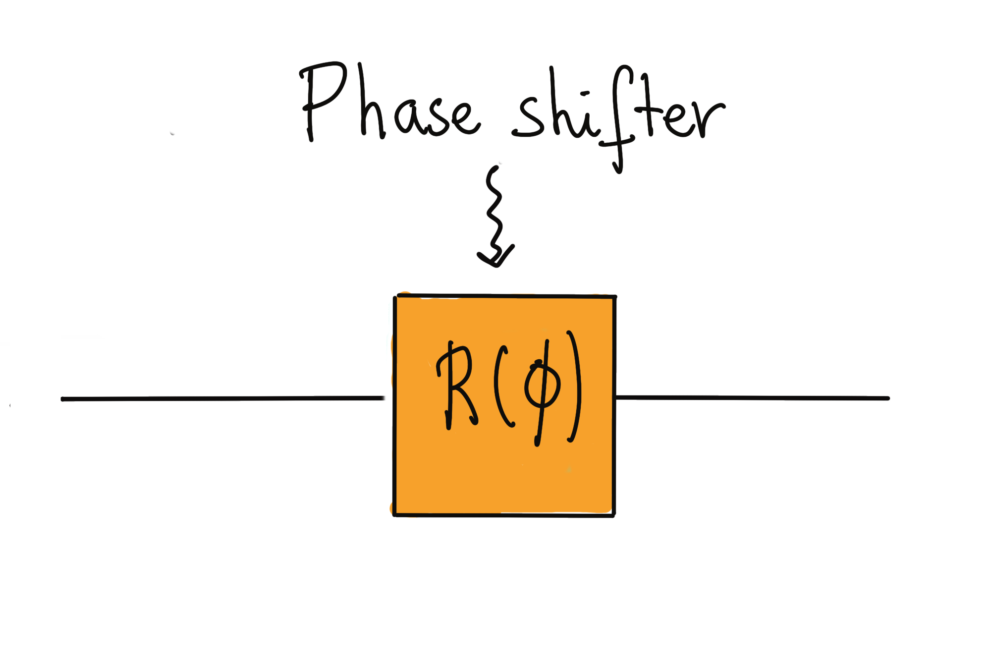
Rotation		Hadamard gate for \(\phi=\frac{\pi}{2}.\)
Continuous variable CNOT		The squeezing parameter is given by \(r=\sinh^{-1}(1/2)\) and the beamsplitters have \(T=\frac{1}{4}(1-\tanh(r)).\) Applies a Control-Z operation on the GKP states when \(\phi = 0\) and a CNOT operation when \(\phi=\pi/2.\)
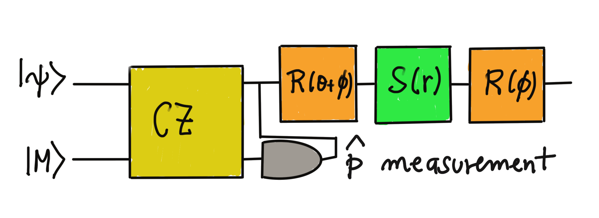
Magic state teleportation		We use an auxiliary magic state \(\vert M\rangle,\) which is the GKP state \(\vert M\rangle = \vert +\rangle +e^{i\pi/4} \vert -\rangle,\) and a \(\hat{P}\) homodyne measurement. If we measure \(\vert -\rangle,\) we apply the shown rotations and squeezers with \(r=\cosh^{-1}(3/4),\) \(\theta=\tan^{-1}(1/2),\) and \(\phi=-\pi/2-\theta,\) resulting in a GKP T gate.

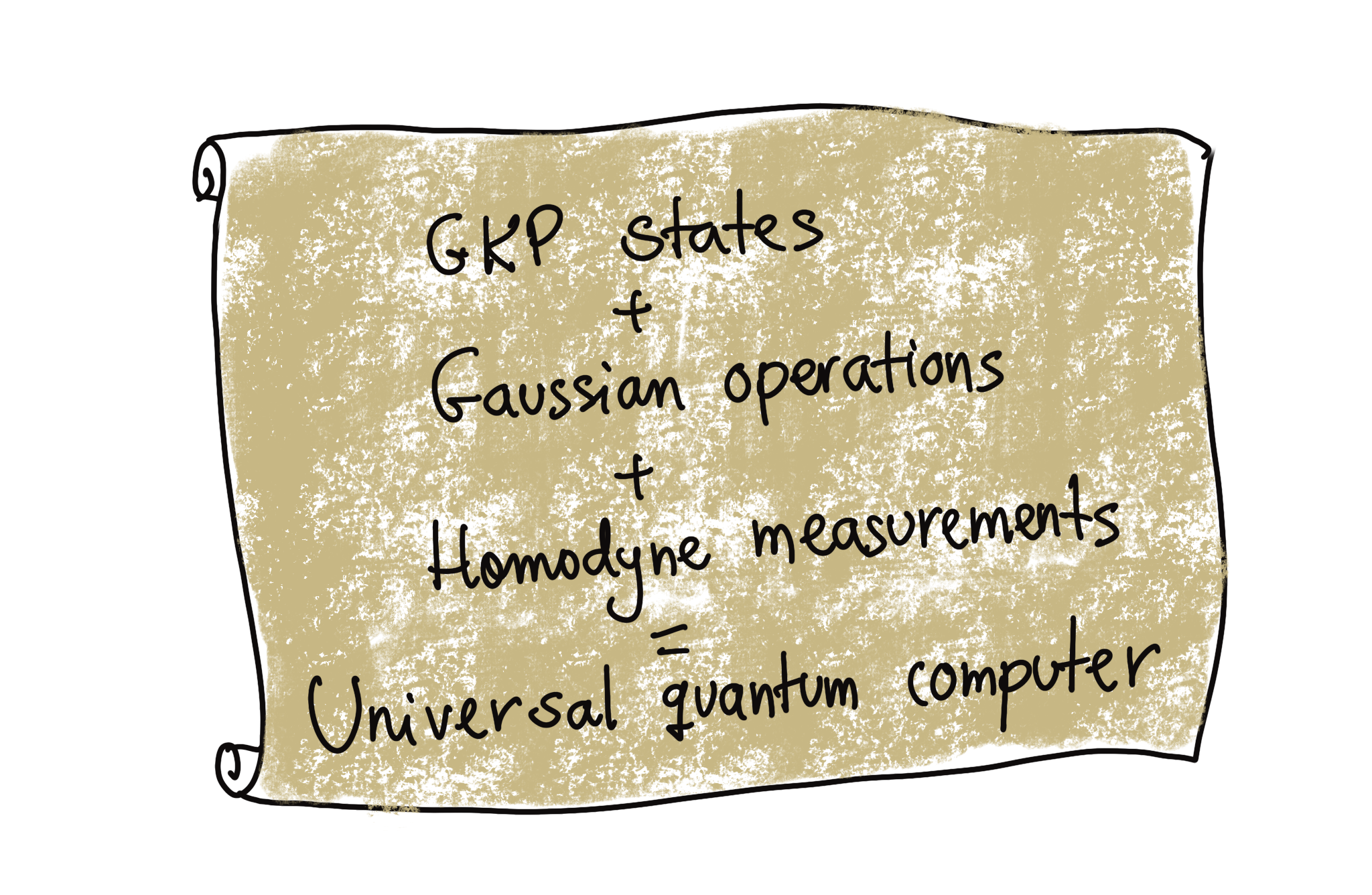
Even if their effect is approximate, these gates are quick and quite straightforward to implement with our current technology. Therefore, we have all the ingredients to build a universal quantum computer using photons, summarized in the formula (see this medium article):

The state of the art

We have now learned the basics of how to build a quantum computer using photonics. So what challenges are there to overcome for scaling further? Let us analyze what we have learned in terms of Di Vincenzo’s criteria, so we can understand what Xanadu is doing to achieve the ambitious goal of building a million-qubit quantum computer.

Looking at the first criterion, we already know that our qubits are far from perfect. Photonics rely on imperfect realizations of GKP states, which in turn makes quantum computations only approximate. Moreover, while we know a lot about GKP states, it is not easy to characterize them after taking into account the noise, so the qubits are not as well-defined as we would like. But our qubits are scalable: GBS circuits can be built on small chips, which we can stack and connect together using optical fibers. Moreover, compared to other implementations where low temperatures are needed everywhere, in photonic quantum computers we only need them for the PNRs to work. Since cryogenics are a bulky part of quantum computing architectures, photonic technology promises to be more scalable than, for example, trapped ion or superconducting devices.

The second criterion, the ability to prepare a qubit, is clearly a challenge. We need GKP states, but these cannot be prepared deterministically; we need to get a bit lucky. We can bypass this by multiplexing, that is, using many Gaussian Boson Sampling circuits in parallel. Moreover, higher-quality GKP states need larger circuits, which in turn can decrease the probability of qubit production. How can we try to solve this? Xanadu is currently following a hybrid approach. When we fail to produce a GKP state, Xanadu’s architecture produces squeezed states using a separate squeezer. Strongly-entangled squeezed states are a precious resource, since other encodings beyond GKP allow us to use these states as a resource for (non-universal) quantum computing 11.

The third criterion of long decoherence times seems innocuous at a first glance. However, although the quantum state of individual photons is robust, we do need to minimize the number of photons that escape to the environment. Recall that all quantum states of light are superpositions of Fock states. If a photon escapes, our state changes! The technology for the minimization of photon loss has come a long way, but it’s not perfect yet. We can avoid losses by optimizing the depth of our circuits, so that photons have a smaller probability of escaping. The GKP encoding also works in our favour, since it is robust against noise and small displacements from GKP states can be easily steered back.

The fourth criterion is pretty much satisfied by photonic quantum computers. We have seen that we can perform universal computations using Gaussian operations, provided that we have GKP states. Barring our imperfect qubits, quantum computing gates are straightforward to implement with good precision inside a chip. Moreover, entangling photons is relatively easy using common optical devices, as opposed to other technologies that rely on rather complicated and slow gates.

Finally, we need to be able to measure qubits. Homodyne detection can be done easily and with great precision. In general, we do not need to measure the number of photons at the end of a quantum computation, quadrature measurement is enough to distinguish quantum states. The fancy PNRs are only required for qubit production!

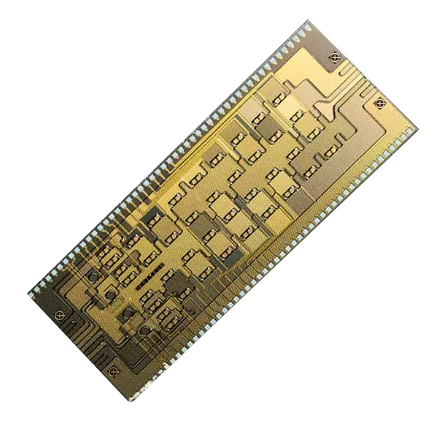
Xanadu’s X8 Gaussian Boson Sampling chip. Variants of this chip can be used to generate approximate GKP states.

Conclusion

The approach of photonic devices to quantum computing is quite different from other technologies. Recent theoretical and technological developments have given a boost to their status as a scalable approach, although the generation of qubits remains a challenge to overcome. The variety of ways that we can encode qubits into photonic states leave plenty of room for creativity, and opens the door for further research and engineering breakthroughs. If you would like to learn more about photonics, make sure to check out the Strawberry Fields demos, as well as the references listed below.

References

1

D. DiVincenzo. (2000) “The Physical Implementation of Quantum Computation”, Fortschritte der Physik 48 (9–11): 771–783. (arXiv)

2

C. Weedbrook, et al. (2012) “Gaussian Quantum Information”, Rev. Mod. Phys. 84, 621. (arXiv)

3

S. Sabouri, et al. (2021) “Thermo Optical Phase Shifter With Low Thermal Crosstalk for SOI Strip Waveguide” IEEE Photonics Journal vol. 13, no. 2, 6600112.

4

M. Paris. (1996) “Displacement operator by beam splitter”, Physics Letters A, 217 (2-3): 78-80.

5(1,2,3)

S. Braunstein, P. van Loock. (2005) “Quantum information with continuous variables”, Rev. Mod. Phys. 77, 513. (arXiv)

6

C. Hamilton , et al. (2017) “Gaussian Boson Sampling”, Phys. Rev. Lett. 119, 170501. (arXiv)

7

H.S. Zhong, et al. (2020) “Quantum computational advantage using photons”, Science 370, 6523: 1460-1463. (arXiv)

8

L. Madsen, et al. (2022) “Quantum computational advantage with a programmable photonic processor” Nature 606, 75-81.

9(1,2,3)

I. Tzitrin, et al. (2020) “Progress towards practical qubit computation using approximate Gottesman-Kitaev-Preskill codes” Phys. Rev. A 101, 032315. (arXiv)

10

D. Gotesman, A. Kitaev, J. Preskill. (2001) “Encoding a qubit in an oscillator”, Phys. Rev. A 64, 012310. (arXiv)

11(1,2)

E. Bourassa, et al. (2021) “Blueprint for a Scalable Photonic Fault-Tolerant Quantum Computer”, Quantum 5, 392. (arXiv)

About the author

Alvaro Ballon

Alvaro is a quantum computing educator at Xanadu. His work involves making the latest developments in quantum computing accessible to the community.

demos/tutorial_photonics

 

Download Python script

 

Download Notebook

 

View on GitHub