Error mitigation with Mitiq and PennyLane

Authors: Tom Bromley (PennyLane) and Andrea Mari (Mitiq) — Posted: 29 November 2021. Last updated: 29 November 2021.

Have you ever run a circuit on quantum hardware and not quite got the result you were expecting? If so, welcome to the world of noisy intermediate-scale quantum (NISQ) devices! These devices must function in noisy environments and are unable to execute quantum circuits perfectly, resulting in outputs that can have a significant error. The long-term plan of quantum computing is to develop a subsequent generation of error-corrected hardware. In the meantime, how can we best utilize our error-prone NISQ devices for practical tasks? One proposed solution is to adopt an approach called error mitigation, which aims to minimize the effects of noise by executing a family of related circuits and using the results to estimate an error-free value.

This demo shows how error mitigation can be carried out by combining PennyLane with the Mitiq package, a Python-based library providing a range of error mitigation techniques. Integration with PennyLane is available from the 0.11 version of Mitiq, which can be installed using

pip install "mitiq>=0.11"

We’ll begin the demo by jumping straight into the deep end and seeing how to mitigate a simple noisy circuit in PennyLane with Mitiq as a backend. After, we’ll take a step back and discuss the theory behind the error mitigation approach we used, known as zero-noise extrapolation. Using this knowledge, we’ll give a more detailed explanation of how error mitigation can be carried out in PennyLane. The final part of this demo showcases the application of mitigation to quantum chemistry, allowing us to more accurately calculate the potential energy surface of molecular hydrogen.

Mitigating noise in a simple circuit

We first need a noisy device to execute our circuit on. Let’s keep things simple for now by loading the default.mixed simulator and artificially adding PhaseDamping noise.

import pennylane as qml

n_wires = 4

# Describe noise
noise_gate = qml.PhaseDamping
noise_strength = 0.1

# Load devices
dev_ideal = qml.device("default.mixed", wires=n_wires)
dev_noisy = qml.transforms.insert(noise_gate, noise_strength)(dev_ideal)

In the above, we load a noise-free device dev_ideal and a noisy device dev_noisy, which is constructed from the qml.transforms.insert transform. This transform works by intercepting each circuit executed on the device and adding the PhaseDamping noise channel directly after every gate in the circuit. To get a better understanding of noise channels like PhaseDamping, check out the Noisy circuits tutorial.

The next step is to define our circuit. Inspired by the mirror circuits concept introduced by Proctor et al. 1 let’s fix a circuit that applies a unitary \(U\) followed by its inverse \(U^{\dagger}\), with \(U\) given by the SimplifiedTwoDesign template. We also fix a measurement of the PauliZ observable on our first qubit. Importantly, such a circuit performs an identity transformation \(U^{\dagger} U |\psi\rangle = |\psi\rangle\) to any input state \(|\psi\rangle\) and we can show that the expected value of an ideal circuit execution with an input state \(|0\rangle\) is

\[\langle 0 | U U^{\dagger} Z U^{\dagger} U | 0 \rangle = 1.\]

Although this circuit seems trivial, it provides an ideal test case for benchmarking noisy devices where we expect the output to be less than one due to the detrimental effects of noise. Let’s check this out in PennyLane code:

from pennylane import numpy as np

np.random.seed(1967)

# Select template to use within circuit and generate parameters
n_layers = 1
template = qml.SimplifiedTwoDesign
weights_shape = template.shape(n_layers, n_wires)
w1, w2 = [2 * np.pi * np.random.random(s) for s in weights_shape]


def circuit(w1, w2):
    template(w1, w2, wires=range(n_wires))
    qml.adjoint(template)(w1, w2, wires=range(n_wires))
    return qml.expval(qml.PauliZ(0))


ideal_qnode = qml.QNode(circuit, dev_ideal)
noisy_qnode = qml.QNode(circuit, dev_noisy)

First, we’ll visualize the circuit:

print(qml.draw(ideal_qnode, expansion_strategy="device")(w1, w2))

Out:

0: ──RY(4.56)─╭●──RY(5.93)──RY(-5.93)────────────────────────────────────╭●──RY(-4.56)─┤  <Z>
1: ──RY(3.60)─╰Z──RY(5.90)─╭●──────────RY(5.18)──RY(-5.18)─╭●──RY(-5.90)─╰Z──RY(-3.60)─┤
2: ──RY(4.05)─╭●──RY(3.32)─╰Z──────────RY(1.07)──RY(-1.07)─╰Z──RY(-3.32)─╭●──RY(-4.05)─┤
3: ──RY(3.51)─╰Z──RY(3.66)──RY(-3.66)────────────────────────────────────╰Z──RY(-3.51)─┤

As expected, executing the circuit on an ideal noise-free device gives a result of 1.

ideal_qnode(w1, w2)

Out:

tensor(1., requires_grad=True)

On the other hand, we obtain a noisy result when running on dev_noisy:

noisy_qnode(w1, w2)

Out:

tensor(0.71729164, requires_grad=True)

So, we have set ourselves up with a benchmark circuit and seen that executing on a noisy device gives imperfect results. Can the results be improved? Time for error mitigation! We’ll first show how easy it is to add error mitigation in PennyLane with Mitiq as a backend, before explaining what is going on behind the scenes.

Note

To run the code below you will need to have the Qiskit plugin installed. This plugin can be installed using:

pip install pennylane-qiskit

The Qiskit plugin is required to convert our PennyLane circuits to OpenQASM 2.0, which is used as an intermediate representation when working with Mitiq.

from mitiq.zne.scaling import fold_global
from mitiq.zne.inference import RichardsonFactory
from pennylane.transforms import mitigate_with_zne

extrapolate = RichardsonFactory.extrapolate
scale_factors = [1, 2, 3]

mitigated_qnode = mitigate_with_zne(scale_factors, fold_global, extrapolate)(
    noisy_qnode
)
mitigated_qnode(w1, w2)

Out:

0.898519654741083

Amazing! Using PennyLane’s mitigate_with_zne transform, we can create a new mitigated_qnode whose result is closer to the ideal noise-free value of 1. How does this work?

Understanding error mitigation

Error mitigation can be realized through a number of techniques, and the Mitiq documentation is a great resource to start learning more. In this demo, we focus upon the zero-noise extrapolation (ZNE) method originally introduced by Temme et al. 2 and Li et al. 3.

The ZNE method works by assuming that the amount of noise present when a circuit is run on a noisy device is enumerated by a parameter \(\gamma\). Suppose we have an input circuit that experiences an amount of noise \(\gamma = \gamma_{0}\) when executed. Ideally, we would like to evaluate the result of the circuit in the \(\gamma = 0\) noise-free setting.

To do this, we create a family of equivalent circuits whose ideal noise-free value is the same as our input circuit. However, when run on a noisy device, each circuit experiences an amount of noise \(\gamma = s \gamma_{0}\) for some scale factor \(s \ge 1\). By evaluating the noisy outputs of each circuit, we can extrapolate to \(s=0\) to estimate the result of running a noise-free circuit.

A key element of ZNE is the ability to run equivalent circuits for a range of scale factors \(s\). When the noise present in a circuit scales with the number of gates, \(s\) can be varied using unitary folding 4. Unitary folding works by noticing that any unitary \(V\) is equivalent to \(V V^{\dagger} V\). This type of transform can be applied to individual gates in the circuit or to the whole circuit. Let’s see how folding works in code using Mitiq’s fold_global function, which folds globally by setting \(V\) to be the whole circuit. We begin by making a copy of our above circuit using a QuantumTape, which provides a low-level approach for circuit construction in PennyLane.

with qml.tape.QuantumTape() as circuit:
    template(w1, w2, wires=range(n_wires))
    qml.adjoint(template)(w1, w2, wires=range(n_wires))

Don’t worry, in most situations you will not need to work with a PennyLane QuantumTape! We are just dropping down to this representation to gain a greater understanding of the Mitiq integration. Let’s see how folding works for some typical scale factors:

scale_factors = [1, 2, 3]
folded_circuits = [fold_global(circuit, scale_factor=s) for s in scale_factors]

for s, c in zip(scale_factors, folded_circuits):
    print(f"Globally-folded circuit with a scale factor of {s}:")
    print(qml.drawer.tape_text(c, decimals=2, max_length=80))

Out:

Globally-folded circuit with a scale factor of 1:
0: ──RY(4.56)─╭●──RY(5.93)──RY(-5.93)────────────────────────────────────╭●
1: ──RY(3.60)─╰Z──RY(5.90)─╭●──────────RY(5.18)──RY(-5.18)─╭●──RY(-5.90)─╰Z
2: ──RY(4.05)─╭●──RY(3.32)─╰Z──────────RY(1.07)──RY(-1.07)─╰Z──RY(-3.32)─╭●
3: ──RY(3.51)─╰Z──RY(3.66)──RY(-3.66)────────────────────────────────────╰Z

───RY(-4.56)─┤
───RY(-3.60)─┤
───RY(-4.05)─┤
───RY(-3.51)─┤
Globally-folded circuit with a scale factor of 2:
0: ──RY(4.56)─╭●──RY(5.93)──RY(-5.93)────────────────────────────────────╭●
1: ──RY(3.60)─╰Z──RY(5.90)─╭●──────────RY(5.18)──RY(-5.18)─╭●──RY(-5.90)─╰Z
2: ──RY(4.05)─╭●──RY(3.32)─╰Z──────────RY(1.07)──RY(-1.07)─╰Z──RY(-3.32)─╭●
3: ──RY(3.51)─╰Z──RY(3.66)──RY(-3.66)────────────────────────────────────╰Z

───RY(-4.56)──RY(4.56)─╭●───────────────────────────────────────────────────────
───RY(-3.60)──RY(3.60)─╰Z──RY(5.90)─╭●──RY(5.18)──RY(-5.18)──RY(5.18)──RY(-5.18)
───RY(-4.05)──RY(4.05)─╭●──RY(3.32)─╰Z──RY(1.07)──RY(-1.07)──RY(1.07)──RY(-1.07)
───RY(-3.51)──RY(3.51)─╰Z───────────────────────────────────────────────────────

────────────────╭●──RY(-4.56)─┤
──╭●──RY(-5.90)─╰Z──RY(-3.60)─┤
──╰Z──RY(-3.32)─╭●──RY(-4.05)─┤
────────────────╰Z──RY(-3.51)─┤
Globally-folded circuit with a scale factor of 3:
0: ──RY(4.56)─╭●──RY(5.93)──RY(-5.93)────────────────────────────────────╭●
1: ──RY(3.60)─╰Z──RY(5.90)─╭●──────────RY(5.18)──RY(-5.18)─╭●──RY(-5.90)─╰Z
2: ──RY(4.05)─╭●──RY(3.32)─╰Z──────────RY(1.07)──RY(-1.07)─╰Z──RY(-3.32)─╭●
3: ──RY(3.51)─╰Z──RY(3.66)──RY(-3.66)────────────────────────────────────╰Z

───RY(-4.56)──RY(4.56)─╭●──RY(5.93)──RY(-5.93)────────────────────────
───RY(-3.60)──RY(3.60)─╰Z──RY(5.90)─╭●──────────RY(5.18)──RY(-5.18)─╭●
───RY(-4.05)──RY(4.05)─╭●──RY(3.32)─╰Z──────────RY(1.07)──RY(-1.07)─╰Z
───RY(-3.51)──RY(3.51)─╰Z──RY(3.66)──RY(-3.66)────────────────────────

─────────────╭●──RY(-4.56)──RY(4.56)─╭●──RY(5.93)──RY(-5.93)──────────
───RY(-5.90)─╰Z──RY(-3.60)──RY(3.60)─╰Z──RY(5.90)─╭●──────────RY(5.18)
───RY(-3.32)─╭●──RY(-4.05)──RY(4.05)─╭●──RY(3.32)─╰Z──────────RY(1.07)
─────────────╰Z──RY(-3.51)──RY(3.51)─╰Z──RY(3.66)──RY(-3.66)──────────

───────────────────────────╭●──RY(-4.56)─┤
───RY(-5.18)─╭●──RY(-5.90)─╰Z──RY(-3.60)─┤
───RY(-1.07)─╰Z──RY(-3.32)─╭●──RY(-4.05)─┤
───────────────────────────╰Z──RY(-3.51)─┤

Although these circuits are a bit deep, if you look carefully, you might be able to convince yourself that they are all equivalent! In fact, since we have fixed our original circuit to be of the form \(U U^{\dagger}\), we get:

• When the scale factor is \(s=1\), the resulting circuit is

  \[V = U^{\dagger} U = \mathbb{I}.\]

  Hence, the \(s=1\) setting gives us the original unfolded circuit.

• When \(s=3\), the resulting circuit is

  \[V V^{\dagger} V = U^{\dagger} U U U^{\dagger} U^{\dagger} U = \mathbb{I}.\]

  In other words, we fold the whole circuit once when \(s=3\). Generally, whenever \(s\) is an odd integer, we fold \((s - 1) / 2\) times.

• The \(s=2\) setting is a bit more subtle. Now we apply folding only to the second half of the circuit, which is in our case given by \(U^{\dagger}\). The resulting partially-folded circuit is

  \[(U^{\dagger} U U^{\dagger}) U = \mathbb{I}.\]

  Visit Ref. 4 to gain a deeper understanding of unitary folding.

If you’re still not convinced, we can evaluate the folded circuits on our noise-free device dev_ideal. To do this, we’ll define an executor function that adds the PauliZ measurement onto the first qubit of each input circuit and then runs the circuits on a target device.

def executor(circuits, dev=dev_noisy):
    # Support both a single circuit and multiple circuit execution
    circuits = [circuits] if isinstance(circuits, qml.tape.QuantumTape) else circuits

    circuits_with_meas = []

    # Loop through circuits and add on measurement
    for c in circuits:
        with qml.tape.QuantumTape() as circuit_with_meas:
            for o in c.operations:
                qml.apply(o)
            qml.expval(qml.PauliZ(0))
        circuits_with_meas.append(circuit_with_meas)

    return qml.execute(circuits_with_meas, dev, gradient_fn=None)

We need to do this step as part of the Mitiq integration with the low-level PennyLane QuantumTape. You will not have to worry about these details when using the main mitigate_with_zne function we encountered earlier.

Now, let’s execute these circuits:

executor(folded_circuits, dev=dev_ideal)

Out:

[tensor(1., requires_grad=True), tensor(1., requires_grad=True), tensor(1., requires_grad=True)]

By construction, these circuits are equivalent to the original and have the same output value of \(1\). On the other hand, each circuit has a different depth. If we expect each gate in a circuit to contribute an amount of noise when running on NISQ hardware, we should see the result of the executed circuit degrade with increased depth. This can be confirmed using the dev_noisy device

executor(folded_circuits, dev=dev_noisy)

Out:

[tensor(0.71729164, requires_grad=True), tensor(0.54368629, requires_grad=True), tensor(0.3777036, requires_grad=True)]

Although this degradation may seem undesirable, it is part of the standard recipe for ZNE error mitigation: we have a family of equivalent circuits that experience a varying amount of noise when executed on hardware, and we are able to control the amount of noise by varying the folding scale factor \(s\) which determines the circuit depth. The final step is to extrapolate our results back to \(s=0\), providing us with an estimate of the noise-free result of the circuit.

Performing extrapolation is a well-studied numeric method in mathematics, and Mitiq provides access to some of the core approaches. Here we use the Richardson extrapolation method with the objective of finding a curve \(y = f(x)\) with some fixed \((x, y)\) values given by the scale factors and corresponding circuit execution results, respectively. This can be performed using:

# Evaluate noise-scaled expectation values
noisy_expectation_values = executor(folded_circuits, dev=dev_noisy)

# Initialize extrapolation method
fac = RichardsonFactory(scale_factors)

# Load data into extrapolation factory
for x, y in zip(scale_factors, noisy_expectation_values):
    fac.push({"scale_factor": x}, y)

# Run extrapolation
zero_noise = fac.reduce()

print(f"ZNE result: {zero_noise}")

Out:

ZNE result: 0.898519654741083

Let’s make a plot of the data and fitted extrapolation function.

_ = fac.plot_fit()

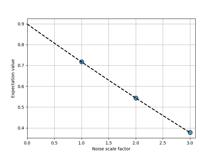
Since we are using the Richardson extrapolation method, the fitted function (dashed line) corresponds to a polynomial interpolation of the measured data (blue points).

The zero-noise limit corresponds to the value of the extrapolation function evaluated at x=0.

Error mitigation in PennyLane

Now that we understand the ZNE method for error mitigation, we can provide a few more details on how it can be performed using PennyLane. As we have seen, the mitigate_with_zne function provides the main entry point. This function is an example of a circuit transform, and it can be applied to pre-constructed QNodes as well as being used as a decorator when constructing new QNodes. For example, suppose we have a qnode already defined. A mitigated QNode can be created using:

mitigated_qnode = mitigate_with_zne(scale_factors, folding, extrapolate)(qnode)

When using mitigate_with_zne, we must specify the target scale factors as well as provide functions for folding and extrapolation. Due to PennyLane’s integration with Mitiq, it is possible to use the folding functions provided in the mitiq.zne.scaling.folding module. For extrapolation, one can use the extrapolate method of the factories in the mitiq.zne.inference module.

We now provide an example of how mitigate_with_zne can be used when constructing a QNode:

from mitiq.zne.scaling import fold_gates_at_random as folding

extrapolate = RichardsonFactory.extrapolate


@mitigate_with_zne(scale_factors, folding, extrapolate, reps_per_factor=100)
@qml.qnode(dev_noisy)
def mitigated_qnode(w1, w2):
    template(w1, w2, wires=range(n_wires))
    qml.adjoint(template)(w1, w2, wires=range(n_wires))
    return qml.expval(qml.PauliZ(0))


mitigated_qnode(w1, w2)

Out:

0.9545857750970078

In the above, we can easily add in error mitigation using the @mitigate_with_zne decorator. To keep things interesting, we’ve swapped out our folding function to instead perform folding on randomly-selected gates. Whenever the folding function is stochastic, there will not be a unique folded circuit corresponding to a given scale factor. For example, the following three distinct circuits are all folded with a scale factor of \(s=1.1\):

for _ in range(3):
    print(qml.drawer.tape_text(folding(circuit, scale_factor=1.1), decimals=2, max_length=80))

Out:

0: ──RY(4.56)─╭●──RY(5.93)──RY(-5.93)──────────────────────────────────────────
1: ──RY(3.60)─╰Z──RY(5.90)─╭●──────────RY(5.18)──RY(-5.18)─────────────────────
2: ──RY(4.05)─╭●──RY(3.32)─╰Z──────────RY(1.07)──RY(-1.07)──RY(1.07)──RY(-1.07)
3: ──RY(3.51)─╰Z──RY(3.66)──RY(-3.66)──────────────────────────────────────────

────────────────╭●──RY(-4.56)─┤
──╭●──RY(-5.90)─╰Z──RY(-3.60)─┤
──╰Z──RY(-3.32)─╭●──RY(-4.05)─┤
────────────────╰Z──RY(-3.51)─┤
0: ──RY(4.56)─╭●──RY(5.93)──RY(-5.93)─────────────────────────────────────────
1: ──RY(3.60)─╰Z──RY(5.90)─╭●──────────RY(5.18)──RY(-5.18)─╭●─╭●─╭●──RY(-5.90)
2: ──RY(4.05)─╭●──RY(3.32)─╰Z──────────RY(1.07)──RY(-1.07)─╰Z─╰Z─╰Z──RY(-3.32)
3: ──RY(3.51)─╰Z──RY(3.66)──RY(-3.66)─────────────────────────────────────────

──╭●──RY(-4.56)─┤
──╰Z──RY(-3.60)─┤
──╭●──RY(-4.05)─┤
──╰Z──RY(-3.51)─┤
0: ──RY(4.56)─╭●──RY(5.93)──RY(-5.93)──────────────────────────────────────────
1: ──RY(3.60)─╰Z──RY(5.90)─╭●──────────RY(5.18)──RY(-5.18)──RY(5.18)──RY(-5.18)
2: ──RY(4.05)─╭●──RY(3.32)─╰Z──────────RY(1.07)──RY(-1.07)─────────────────────
3: ──RY(3.51)─╰Z──RY(3.66)──RY(-3.66)──────────────────────────────────────────

────────────────╭●──RY(-4.56)─┤
──╭●──RY(-5.90)─╰Z──RY(-3.60)─┤
──╰Z──RY(-3.32)─╭●──RY(-4.05)─┤
────────────────╰Z──RY(-3.51)─┤

To accommodate for this randomness, we can perform multiple repetitions of random folding for a fixed \(s\) and average over the execution results to generate the value \(f(s)\) used for extrapolation. As shown above, the number of repetitions is controlled by setting the optional reps_per_factor argument.

We conclude this section by highlighting the possibility of working directly with the core functionality available in Mitiq. For example, the execute_with_zne function is one of the central components of ZNE support in Mitiq and is compatible with circuits constructed using a PennyLane QuantumTape. Working directly with Mitiq can be preferable when more flexibility is required in specifying the error mitigation protocol. For example, the code below shows how an adaptive approach can be used to determine a sequence of scale factors for extrapolation using Mitiq’s AdaExpFactory.

from mitiq.zne import execute_with_zne
from mitiq.zne.inference import AdaExpFactory

factory = AdaExpFactory(steps=20)

execute_with_zne(circuit, executor, factory=factory, scale_noise=fold_global)

Out:

0.9589759281849715

Recall that circuit is a PennyLane QuantumTape and that it should not include measurements. We also use the executor function defined earlier that adds on the target measurement and executes on a noisy device.

Mitigating noisy circuits in quantum chemistry

We’re now ready to apply our knowledge to a more practical problem in quantum chemistry: calculating the potential energy surface of molecular hydrogen. This is achieved by finding the ground state energy of \(H_{2}\) as we increase the bond length between the hydrogen atoms. As shown in this tutorial, one approach to finding the ground state energy is to calculate the corresponding qubit Hamiltonian and to fix an ansatz variational quantum circuit that returns its expectation value. We can then vary the parameters of the circuit to minimize the energy.

To find the potential energy surface of \(H_{2}\), we must choose a range of interatomic distances and calculate the qubit Hamiltonian corresponding to each distance. We then optimize the variational circuit with a new set of parameters for each Hamiltonian and plot the resulting energies for each distance. In this demo, we compare the potential energy surface reconstructed when the optimized variational circuits are run on ideal, noisy, and noise-mitigated devices.

Instead of modifying the default.mixed device to add simple noise as we do above, let’s choose a noise model that is a little closer to physical hardware. Suppose we want to simulate the ibmq_lima hardware device available on IBMQ. We can load a noise model that represents this device using:

from qiskit.test.mock import FakeLima
from qiskit.providers.aer.noise import NoiseModel

backend = FakeLima()
noise_model = NoiseModel.from_backend(backend)

Out:

/home/runner/work/qml/qml/demonstrations/tutorial_error_mitigation.py:432: DeprecationWarning: The module 'qiskit.test.mock' is deprecated since Qiskit Terra 0.21.0, and will be removed 3 months or more later. Instead, you should import the desired object directly 'qiskit.providers.fake_provider'.
  from qiskit.test.mock import FakeLima

We can then set up our ideal device and the noisy simulator of ibmq_lima.

n_wires = 4

dev_ideal = qml.device("default.qubit", wires=n_wires)
dev_noisy = qml.device(
    "qiskit.aer",
    wires=n_wires,
    noise_model=noise_model,
    optimization_level=0,
    shots=10000,
)

Note the use of the optimization_level=0 argument when loading the noisy device. This prevents the qiskit.aer transpiler from performing a pre-execution circuit optimization.

To simplify this demo, we will load pre-trained parameters for our variational circuit.

params = np.load("error_mitigation/params.npy")

These parameters can be downloaded by clicking here. We are now ready to set up the variational circuit and run on the ideal and noisy devices.

from pennylane import qchem

# Describe quantum chemistry problem
symbols = ["H", "H"]
distances = np.arange(0.5, 3.0, 0.25)

ideal_energies = []
noisy_energies = []

for r, phi in zip(distances, params):
    # Assume atoms lie on the Z axis
    coordinates = np.array([0.0, 0.0, 0.0, 0.0, 0.0, r])

    # Load qubit Hamiltonian
    H, _ = qchem.molecular_hamiltonian(symbols, coordinates)

    # Define ansatz circuit
    def qchem_circuit(phi):
        qml.PauliX(wires=0)
        qml.PauliX(wires=1)
        qml.DoubleExcitation(phi, wires=range(n_wires))
        return qml.expval(H)

    ideal_energy = qml.QNode(qchem_circuit, dev_ideal)
    noisy_energy = qml.QNode(qchem_circuit, dev_noisy)

    ideal_energies.append(ideal_energy(phi))
    noisy_energies.append(noisy_energy(phi))

An error-mitigated version of the potential energy surface can also be calculated using the following:

mitig_energies = []

for r, phi in zip(distances, params):
    # Assume atoms lie on the Z axis
    coordinates = np.array([0.0, 0.0, 0.0, 0.0, 0.0, r])

    # Load qubit Hamiltonian
    H, _ = qchem.molecular_hamiltonian(symbols, coordinates)

    # Define ansatz circuit
    with qml.tape.QuantumTape() as circuit:
        qml.PauliX(wires=0)
        qml.PauliX(wires=1)
        qml.DoubleExcitation(phi, wires=range(n_wires))

    # Define custom executor that expands Hamiltonian measurement
    # into a linear combination of tensor products of Pauli
    # operators.
    def executor(circuit):

        # Add Hamiltonian measurement to circuit
        with qml.tape.QuantumTape() as circuit_with_meas:
            for o in circuit.operations:
                qml.apply(o)
            qml.expval(H)

        # Expand Hamiltonian measurement into tensor product of
        # of Pauli operators. We get a list of circuits to execute
        # and a postprocessing function to combine the results into
        # a single number.
        circuits, postproc = qml.transforms.hamiltonian_expand(
            circuit_with_meas, group=False
        )
        circuits_executed = qml.execute(circuits, dev_noisy, gradient_fn=None)
        return postproc(circuits_executed)

    mitig_energy = execute_with_zne(circuit, executor, scale_noise=fold_global)
    mitig_energies.append(mitig_energy)

Finally, we can plot the three surfaces and compare:

import matplotlib.pyplot as plt

plt.plot(ideal_energies, label="ideal")
plt.plot(noisy_energies, label="noisy")
plt.plot(mitig_energies, label="mitigated")
plt.xlabel("Bond length (Bohr)")
plt.ylabel("Total energy (Hartree)")
plt.legend()
plt.show()

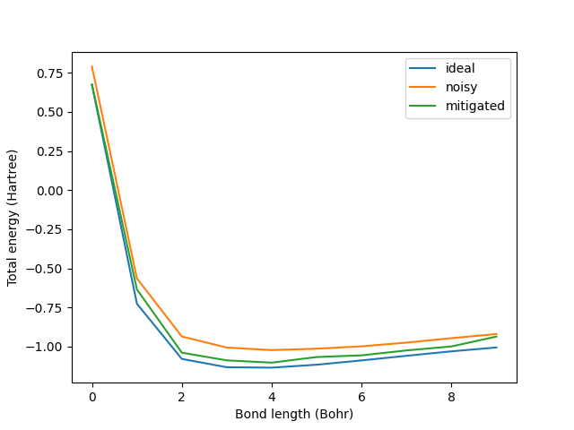
Great, error mitigation has allowed us to more closely approximate the ideal noise-free curve!

We have seen in this demo how easy error mitigation can be in PennyLane when using Mitiq as a backend. As well as understanding the basics of the ZNE method, we have also seen how mitigation can be used to uplift the performance of noisy devices for practical tasks like quantum chemistry. On the other hand, we’ve only just started to scratch the surface of what can be done with error mitigation. We can explore applying the ZNE method to other use cases, or even try out other mitigation methods like probabilistic error cancellation. Let us know where your adventures take you, and the Mitiq and PennyLane teams will keep working to help make error mitigation as easy as possible!

References

1

T. Proctor, K. Rudinger, K. Young, E. Nielsen, R. Blume-Kohout “Measuring the Capabilities of Quantum Computers”, arXiv:2008.11294 (2020).

2

K. Temme, S. Bravyi, J. M. Gambetta “Error Mitigation for Short-Depth Quantum Circuits”, Phys. Rev. Lett. 119, 180509 (2017).

3

Y. Li, S. C. Benjamin “Efficient Variational Quantum Simulator Incorporating Active Error Minimization”, Phys. Rev. X 7, 021050 (2017).

4(1,2)

T. Giurgica-Tiron, Y. Hindy, R. LaRose, A. Mari, W. J. Zeng “Digital zero noise extrapolation for quantum error mitigation”, IEEE International Conference on Quantum Computing and Engineering (2020).

About the authors

Thomas Bromley

Thomas is a quantum scientist working at Xanadu. His work is focused on developing software to execute quantum algorithms on simulators and hardware.

Andrea Mari

Andrea obtained a PhD in quantum information theory from the University of Potsdam (Germany). He worked as a postdoc at Scuola Normale Superiore (Pisa, Italy) and as a remote researcher at Xanadu. Since 2020 is a Member of Technical Staff at Unitary Fund.

demos/tutorial_error_mitigation

 

Download Python script

 

Download Notebook

 

View on GitHub