VQE in different spin sectors

Author: Alain Delgado — Posted: 13 October 2020. Last updated: 25 June 2022.

The Variational Quantum Eigensolver (VQE) algorithm is an approach for finding the lowest-energy state of a molecule using a quantum computer 1.

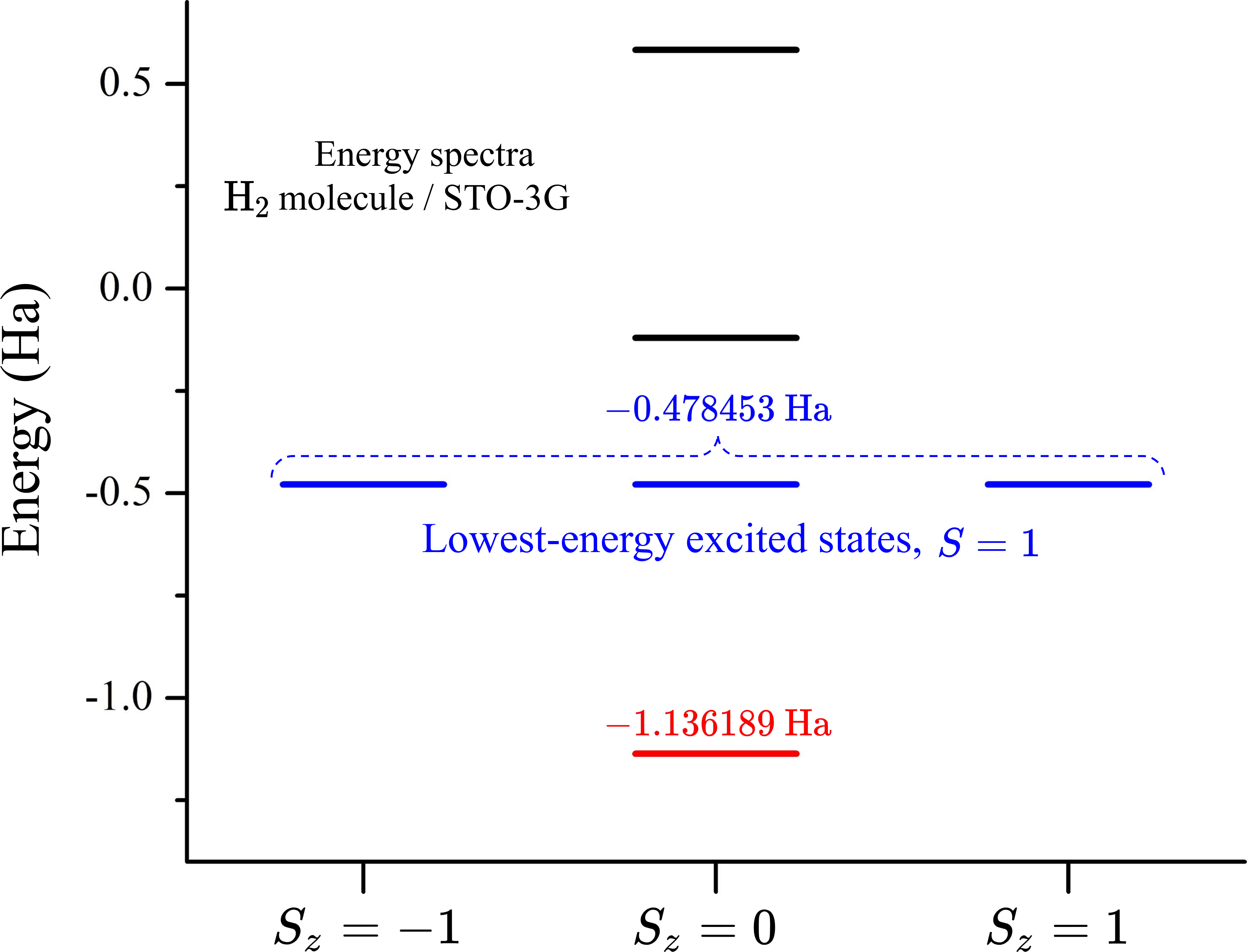
In the absence of spin-orbit coupling, the eigenstates of the molecular Hamiltonian can be calculated for specific values of the spin quantum numbers. This allows us to compute quantities such as the energy of the electronic states in different sectors of the total-spin projection \(S_z\). This is illustrated in the figure below for the energy spectrum of the hydrogen molecule. In this case, the ground state has total spin \(S=0\) while the lowest-lying excited states, with total spin \(S=1\), form a triplet related to the spin components \(S_z=-1, 0, 1\).

In this tutorial we demonstrate how to run VQE simulations to find the lowest-energy states of the hydrogen molecule in different spin sectors. First, we show how to build the electronic Hamiltonian and the total spin operator \(\hat{S}^2\). Next, we use excitation operations, implemented in PennyLane as Givens rotations 2, to prepare the trial states of the molecule. In order to probe the molecular states with different total spin, \(S=0\) and \(S=1\), we apply excitation operations which preserve and modify, respectively, the total-spin projection of the initial state encoded in the qubit register. Finally, we run the VQE algorithm to compute the energy of the states.

Let’s get started!

Building the Hamiltonian and the total spin operator \(\hat{S}^2\)

First, we need to specify the structure of the molecule. This is done by providing a list with the symbols of the constituent atoms and a one-dimensional array with the corresponding nuclear coordinates in atomic units.

from pennylane import numpy as np

symbols = ["H", "H"]
coordinates = np.array([0.0, 0.0, -0.6614, 0.0, 0.0, 0.6614])

The geometry of the molecule can also be imported from an external file using the read_structure() function.

Now, we can build the electronic Hamiltonian. We use a minimal basis set approximation to represent the molecular orbitals. Then, the qubit Hamiltonian of the molecule is built using the molecular_hamiltonian() function.

import pennylane as qml

H, qubits = qml.qchem.molecular_hamiltonian(symbols, coordinates)

print("Number of qubits = ", qubits)
print("The Hamiltonian is ", H)

Out:

Number of qubits =  4
The Hamiltonian is    (-0.2427450126094144) [Z2]
+ (-0.2427450126094144) [Z3]
+ (-0.042072551947439224) [I0]
+ (0.1777135822909176) [Z0]
+ (0.1777135822909176) [Z1]
+ (0.12293330449299361) [Z0 Z2]
+ (0.12293330449299361) [Z1 Z3]
+ (0.16768338855601356) [Z0 Z3]
+ (0.16768338855601356) [Z1 Z2]
+ (0.17059759276836803) [Z0 Z1]
+ (0.1762766139418181) [Z2 Z3]
+ (-0.044750084063019925) [Y0 Y1 X2 X3]
+ (-0.044750084063019925) [X0 X1 Y2 Y3]
+ (0.044750084063019925) [Y0 X1 X2 Y3]
+ (0.044750084063019925) [X0 Y1 Y2 X3]

The outputs of the function are the Hamiltonian and the number of qubits required for the quantum simulations. For the \(\mathrm{H}_2\) molecule in a minimal basis, we have four molecular spin-orbitals, which defines the number of qubits.

The molecular_hamiltonian() function allows us to define additional keyword arguments to simulate more complicated molecules. For more details take a look at the tutorial Building molecular Hamiltonians.

We also want to build the total spin operator \(\hat{S}^2\),

\[\hat{S}^2 = \frac{3}{4} N + \sum_{\alpha, \beta, \gamma, \delta} \langle \alpha, \beta \vert \hat{s}_1 \cdot \hat{s}_2 \vert \gamma, \delta \rangle ~ \hat{c}_\alpha^\dagger \hat{c}_\beta^\dagger \hat{c}_\gamma \hat{c}_\delta.\]

In the equation above, \(N\) is the number of electrons, \(\hat{c}\) and \(\hat{c}^\dagger\) are respectively the electron annihilation and creation operators, and \(\langle \alpha, \beta \vert \hat{s}_1 \cdot \hat{s}_2 \vert \gamma, \delta \rangle\) is the matrix element of the two-body spin operator \(\hat{s}_1 \cdot \hat{s}_2\) in the basis of spin orbitals.

We use the spin2() function to build the \(\hat{S}^2\) observable.

electrons = 2
S2 = qml.qchem.spin2(electrons, qubits)
print(S2)

Out:

  ((0.375+0j)) [Z0]
+ ((0.375+0j)) [Z1]
+ ((0.375+0j)) [Z2]
+ ((0.375+0j)) [Z3]
+ ((0.75+0j)) [I0]
+ ((-0.375+0j)) [Z0 Z1]
+ ((-0.375+0j)) [Z2 Z3]
+ ((-0.125+0j)) [Z0 Z3]
+ ((-0.125+0j)) [Z1 Z2]
+ ((0.125+0j)) [Z0 Z2]
+ ((0.125+0j)) [Z1 Z3]
+ ((-0.125+0j)) [Y0 X1 X2 Y3]
+ ((-0.125+0j)) [X0 Y1 Y2 X3]
+ ((0.125+0j)) [Y0 X1 Y2 X3]
+ ((0.125+0j)) [Y0 Y1 X2 X3]
+ ((0.125+0j)) [Y0 Y1 Y2 Y3]
+ ((0.125+0j)) [X0 X1 X2 X3]
+ ((0.125+0j)) [X0 X1 Y2 Y3]
+ ((0.125+0j)) [X0 Y1 X2 Y3]

Building the quantum circuit to find the ground state

We build the variational circuit for the ground state of the hydrogen molecule using the SingleExcitation and DoubleExcitation operations which act as Givens rotations on subspaces of two and four qubits, respectively 2. The total number of excitation operations is given by all possible single and double excitations of the Hartree-Fock reference state. The indices of the qubits they act on correspond to the spin-orbitals involved in each excitation. For more details on how to use the excitation operations see the tutorial Givens rotations for quantum chemistry.

First, we use the hf_state() function to generate the vector representing the Hartree-Fock state \(\vert 1100 \rangle\) of the \(\mathrm{H}_2\) molecule.

hf = qml.qchem.hf_state(electrons, qubits)
print(hf)

Out:

[1 1 0 0]

Next, we use the excitations() function to generate all single and double excitations of the Hartree-Fock state. This function allows us to define the keyword argument delta_sz to specify the total-spin projection of the excitations with respect to the reference state. This is illustrated in the figure below.

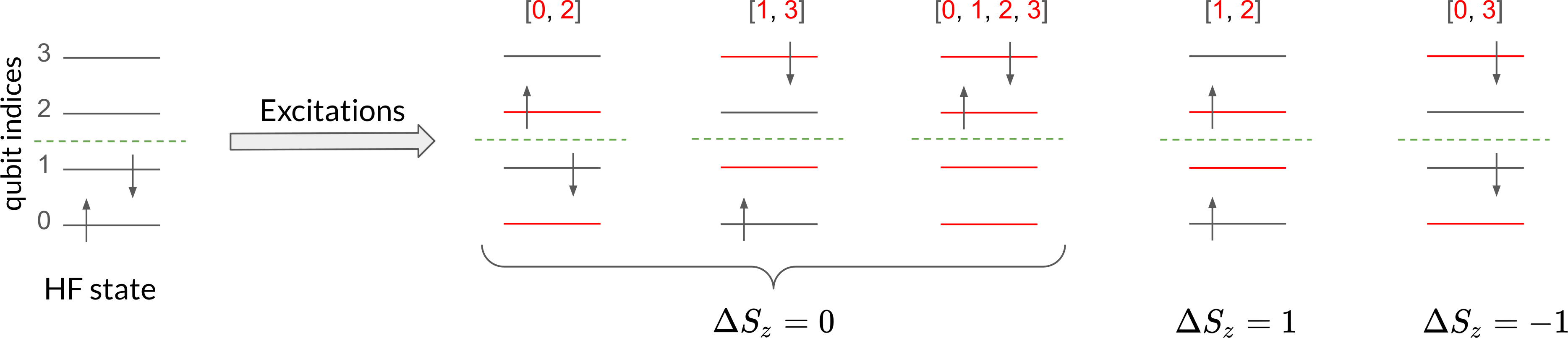
Therefore, for the ground state of the \(\mathrm{H}_2\) molecule we choose delta_sz = 0.

singles, doubles = qml.qchem.excitations(electrons, qubits, delta_sz=0)
print(singles)
print(doubles)

Out:

[[0, 2], [1, 3]]
[[0, 1, 2, 3]]

The output lists singles and doubles contain the qubit indices involved in the single and double excitations. Even and odd indices correspond, respectively, to spin-up and spin-down orbitals. For delta_sz = 0 we have two single excitations, one from qubit 0 to 2 and the other from qubit 1 to 3, and one double excitation from qubits 0, 1 to 2, 3. In order to build the variational circuit, we apply the corresponding excitation operations. This can be done straightforwardly using the AllSinglesDoubles template.

def circuit(params, wires):
    qml.AllSinglesDoubles(params, wires, hf, singles, doubles)

The circuit above prepares trial states for the \(\mathrm{H}_2\) molecule of the form:

\[\vert \Psi(\theta) \rangle = c_\mathrm{HF}(\theta) \vert 1100 \rangle + c_{0123}(\theta) \vert 0011 \rangle + c_{02}(\theta) \vert 0110 \rangle + c_{13}(\theta) \vert 1001 \rangle,\]

where the coefficients \(c\) are functions of the variational parameters \(\theta = (\theta_1, \theta_2, \theta_3)\) to be optimized by the VQE algorithm. Note that the prepared state \(\vert \Psi(\theta) \rangle\) is a superposition of the Hartree-Fock (HF) state with all possible single and double excitations that preserve the spin projection of the HF reference state.

Running the VQE simulation

Now we proceed to optimize the variational parameters. First, we define the device, in this case a qubit simulator:

dev = qml.device("default.qubit", wires=qubits)

Next, we define the cost function as the following QNode, where we make use of the expval() function to compute the expectation value of the hamiltonian. This requires specifying the circuit, the target Hamiltonian, and the device. It returns a cost function that can be evaluated with the circuit parameters:

@qml.qnode(dev, interface="autograd")
def cost_fn(params):
    circuit(params, wires=range(qubits))
    return qml.expval(H)

As a reminder, we also built the total spin operator \(\hat{S}^2\) for which we can now define a function to compute its expectation value:

@qml.qnode(dev, interface="autograd")
def S2_exp_value(params):
    circuit(params, wires=range(qubits))
    return qml.expval(S2)

The total spin \(S\) of the trial state can be obtained from the expectation value \(\langle \hat{S}^2 \rangle\) as

\[S = -\frac{1}{2} + \sqrt{\frac{1}{4} + \langle \hat{S}^2 \rangle}.\]

We define a function to compute the total spin.

def total_spin(params):
    return -0.5 + np.sqrt(1 / 4 + S2_exp_value(params))

Now, we proceed to minimize the cost function to find the ground state. We define the classical optimizer and initialize the circuit parameters.

opt = qml.GradientDescentOptimizer(stepsize=0.8)
np.random.seed(0)  # for reproducibility
theta = np.random.normal(0, np.pi, len(singles) + len(doubles), requires_grad=True)
print(theta)

Out:

[5.54193389 1.25713095 3.07479606]

We carry out the optimization over a maximum of 100 steps, aiming to reach a convergence tolerance of \(10^{-6}\) for the value of the cost function.

max_iterations = 100
conv_tol = 1e-06

for n in range(max_iterations):

    theta, prev_energy = opt.step_and_cost(cost_fn, theta)

    energy = cost_fn(theta)
    spin = total_spin(theta)

    conv = np.abs(energy - prev_energy)

    if n % 4 == 0:
        print(f"Step = {n}, Energy = {energy:.8f} Ha, S = {spin:.4f}")

    if conv <= conv_tol:
        break

print("\n" f"Final value of the ground-state energy = {energy:.8f} Ha")
print("\n" f"Optimal value of the circuit parameters = {theta}")

Out:

Step = 0, Energy = -0.09929557 Ha, S = 0.1014
Step = 4, Energy = -0.87153518 Ha, S = 0.0982
Step = 8, Energy = -1.11692841 Ha, S = 0.0087
Step = 12, Energy = -1.13529755 Ha, S = 0.0004
Step = 16, Energy = -1.13614888 Ha, S = 0.0000
Step = 20, Energy = -1.13618734 Ha, S = 0.0000

Final value of the ground-state energy = -1.13618832 Ha

Optimal value of the circuit parameters = [3.14350662 3.14087516 2.93185886]

As a result, we have estimated the lowest-energy state of the hydrogen molecule with total spin \(S = 0\) which corresponds to the ground state.

Finding the lowest-lying excited state with \(S=1\)

In the last part of the tutorial, we will use VQE to find the lowest-lying excited state of the hydrogen molecule with total spin \(S=1\). In this case, we use the excitations() function to generate excitations whose total-spin projection differs by the quantity delta_sz=1 with respect to the Hartree-Fock state.

singles, doubles = qml.qchem.excitations(electrons, qubits, delta_sz=1)
print(singles)
print(doubles)

Out:

[[1, 2]]
[]

For the \(\mathrm{H}_2\) molecule in a minimal basis set there are no double excitations, but only a spin-flip single excitation from qubit 1 to 2. In this case, the circuit will contain only one SingleExcitation operation. Additionally, as we want to probe the excited state of the hydrogen molecule, we initialize the qubit register to the state \(\vert 0011 \rangle\).

def circuit(params, wires):
    qml.AllSinglesDoubles(params, wires, np.flip(hf), singles, doubles)

This allows us to prepare trial states of the form

\[\vert \Psi(\theta) \rangle = c_{03}(\theta) \vert 0101 \rangle + c_{0123}(\theta) \vert 0011 \rangle,\]

where the first term \(\vert 0101 \rangle\) encodes a spin-flip excitation with \(S_z=-1\) and the second term is a double excitation with \(S_z=0\). Since an eigenstate of the electronic Hamiltonian cannot contain a superposition of states with different total-spin projections, the double excitation coefficient should vanish as the VQE algorithm minimizes the cost function. The optimized state will correspond to the lowest-energy state with spin quantum numbers \(S=1, S_z=-1\).

Now, we define the new functions to compute the expectation values of the Hamiltonian and the total spin operator for the new circuit.

@qml.qnode(dev, interface="autograd")
def cost_fn(params):
    circuit(params, wires=range(qubits))
    return qml.expval(H)


@qml.qnode(dev, interface="autograd")
def S2_exp_value(params):
    circuit(params, wires=range(qubits))
    return qml.expval(S2)

Finally, we generate the new set of initial parameters, and proceed with the VQE algorithm to optimize the variational circuit.

np.random.seed(0)
theta = np.random.normal(0, np.pi, len(singles) + len(doubles), requires_grad=True)

max_iterations = 100
conv_tol = 1e-06

for n in range(max_iterations):

    theta, prev_energy = opt.step_and_cost(cost_fn, theta)

    energy = cost_fn(theta)
    spin = total_spin(theta)

    conv = np.abs(energy - prev_energy)

    if n % 4 == 0:
        print(f"Step = {n}, Energy = {energy:.8f} Ha, S = {spin:.4f}")

    if conv <= conv_tol:
        break

print("\n" f"Final value of the energy = {energy:.8f} Ha")
print("\n" f"Optimal value of the circuit parameters = {theta}")

Out:

Step = 0, Energy = 0.31463319 Ha, S = 0.3539
Step = 4, Energy = -0.38517129 Ha, S = 0.9391
Step = 8, Energy = -0.47698618 Ha, S = 0.9991
Step = 12, Energy = -0.47842743 Ha, S = 1.0000
Step = 16, Energy = -0.47844667 Ha, S = 1.0000

Final value of the energy = -0.47844667 Ha

Optimal value of the circuit parameters = [3.14259046]

As expected, the VQE algorithms has found the lowest-energy state with total spin \(S=1\) which is an excited state of the hydrogen molecule.

Conclusion

In this tutorial we have used the standard VQE algorithm to find the ground and the lowest-lying excited states of the hydrogen molecule. We used the single and double excitation operations, implemented as Givens rotations, to prepare the trial states of a molecule. We also showed how to build the total-spin operator \(\hat{S}^2\) and used it to compute the total spin of the optimized states. By choosing the total-spin projection of the generated excitations, we were able to probe the lowest-energy eigenstates of the molecular Hamiltonian in different sectors of the spin quantum numbers.

References

1

A. Peruzzo, J. McClean et al., “A variational eigenvalue solver on a photonic quantum processor”. Nature Communications 5, 4213 (2014).

2(1,2)

J.M. Arrazola, O. Di Matteo, N. Quesada, S. Jahangiri, A. Delgado, N. Killoran. “Universal quantum circuits for quantum chemistry”. arXiv:2106.13839, (2021)

About the author

Alain Delgado

Alain Delgado Gran is a senior quantum scientist working at Xanadu. He has a background in quantum many-body systems and electronic structure methods. His work focuses on the application of quantum algorithms for simulating advanced materials.

demos/tutorial_vqe_spin_sectors

 

Download Python script

 

Download Notebook

 

View on GitHub