Differentiable pulse programming with qubits in PennyLane

Author: Korbinian Kottmann — Posted: 8 March 2023.

Quantum computers perform gates via electromagnetic pulses on the hardware level. In differentiable pulse programming, we can write quantum algorithms directly on the hardware level and variationally optimize the shape, phase and amplitude of the interactions for our desired goals. In this demo, we are going to introduce pulse programming with qubits in PennyLane and run the ctrl-VQE algorithm 1 on a two-qubit Hamiltonian for the \(\text{HeH}^+\) molecule.

Pulses in quantum computers

In many quantum computing architectures such as superconducting, ion trap and neutral atom Rydberg systems, qubits are realized through physical systems with a discrete set of energy levels. For example, transmon qubits realize an anharmonic oscillator whose ground and first excited states can serve as the two energy levels of a qubit. Such a qubit can be controlled via an electromagnetic field tuned to its energy gap. In general, this electromagnetic field can be altered in time, leading to a time-dependent Hamiltonian \(H(t)\) describing the effect of the field on the qubits. We call driving the system with such an electromagnetic field for a fixed time window \([t_0, t_1]\) a pulse sequence. During a pulse sequence, the state evolves according to the time-dependent Schrödinger equation

\[\frac{d}{dt}|\psi\rangle = -i H(t) |\psi\rangle\]

from an initial state \(|\psi(t_0)\rangle\) to a final state \(|\psi(t_1)\rangle\). This process corresponds to a unitary evolution \(U(t_0, t_1)\) of the input state from time \(t_0\) to \(t_1\), i.e. \(|\psi(t_1)\rangle = U(t_0, t_1) |\psi(t_0)\rangle\).

In most digital quantum computers (with the exception of measurement-based architectures), the amplitude and frequencies of predefined pulse sequences are fine tuned to realize the native gates of the quantum computer. More specifically, the Hamiltonian interaction \(H(t)\) is tuned such that the respective evolution \(U(t_0, t_1)\) realizes for example a Pauli or CNOT gate (see e.g. cross-resonance gates for superconducting qubits in 2).

Pulse programming in PennyLane

A user of a quantum computer typically operates on the higher and more abstract gate level. Future fault-tolerant quantum computers require this abstraction to allow for error correction. For noisy and intermediate-sized quantum computers, the abstraction of decomposing quantum algorithms into a fixed native gate set can be a hindrance and unnecessarily increase execution time, therefore leading to more noise in the computation. The idea of differentiable pulse programming is to optimize quantum circuits on the pulse level instead, with the aim of achieving the shortest interaction sequence a hardware system allows.

In PennyLane, we can simulate arbitrary qubit system interactions to explore the possibilities of such pulse programs. First, we need to define the time-dependent Hamiltonian \(H(p, t)= \sum_i f_i(p_i, t) H_i\) with constant operators \(H_i\) and control fields \(f_i(p_i, t)\). The Hamiltonian depends on the set of parameters \(p = \{p_i\}\). One way to do this in PennyLane is in the following way:

import pennylane as qml
import pennylane.numpy as np
import jax.numpy as jnp
import jax
import matplotlib.pyplot as plt

# Set to float64 precision and remove jax CPU/GPU warning
jax.config.update("jax_enable_x64", True)
jax.config.update("jax_platform_name", "cpu")

def f1(p, t):
    # polyval(p, t) evaluates a polynomial of degree N=len(p)
    # i.e. p[0]*t**(N-1) + p[1]*t**(N-2) + ... + p[N-2]*t + p[N-1]
    return jnp.polyval(p, t)

def f2(p, t):
    return p[0] * jnp.sin(p[1] * t)

Ht = f1 * qml.PauliX(0) + f2 * qml.PauliY(1)

This constructs a ParametrizedHamiltonian. Note that the callable functions f1 and f2 are expected to have the fixed signature (p, t). When calling the ParametrizedHamiltonian, a tuple or list of the parameters for each of the functions is passed in the same order the Hamiltonian was constructed.

p1 = jnp.ones(5)              # parameters for f1
p2 = jnp.array([1.0, jnp.pi]) # parameters for f2
t = 0.5                       # some fixed point in time
print(Ht((p1, p2), t))        # order of parameters p1, p2 matters

Out:

(1.9375*(PauliX(wires=[0]))) + (1.0*(PauliY(wires=[1])))

We can construct general Hamiltonians of the form \(\sum_i H_i^d + \sum_i f_i(p_i, t) H_i\) using qml.dot. Such a time-dependent Hamiltonian consists of time-independent drift terms \(H_i^d\) and time-dependent control terms \(f_i(p_i, t) H_i\) with scalar complex-valued functions \(f_i(p, t).\) In the following we are going to construct \(\sum_i X_i X_{i+1} + \sum_i f_i(p_i, t) Z_i\) with \(f_i(p_i, t) = \sin(p_i^0 t) + \sin(p_i^1 t) \forall i\) as an example:

coeffs = [1.0] * 2
coeffs += [lambda p, t: jnp.sin(p[0] * t) + jnp.sin(p[1] * t) for _ in range(3)]
ops = [qml.PauliX(i) @ qml.PauliX(i + 1) for i in range(2)]
ops += [qml.PauliZ(i) for i in range(3)]

Ht = qml.dot(coeffs, ops)

# random coefficients
key = jax.random.PRNGKey(777)
subkeys = jax.random.split(key, 3) # create list of 3 subkeys
params = [jax.random.uniform(subkeys[i], shape=[2], maxval=5) for i in range(3)]
print(Ht(params, 0.5))

Out:

((1.0*(PauliX(wires=[0]) @ PauliX(wires=[1]))) + (1.0*(PauliX(wires=[1]) @ PauliX(wires=[2])))) + (((1.4456867348869746*(PauliZ(wires=[0]))) + (1.823824746247098*(PauliZ(wires=[1])))) + (1.8206871129031437*(PauliZ(wires=[2]))))

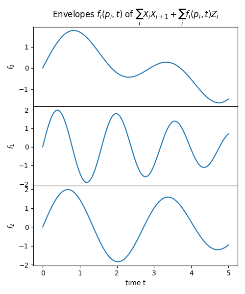
We can visualize the Hamiltonian interaction by plotting the time-dependent envelopes. We refer to the drift term as all constant terms in time, i.e. \(\sum_i X_i X_{i+1}\), and plot the envelopes \(f_i(p_i, t)\) of the time-dependent terms \(f_i(p_i, t) Z_i\).

ts = jnp.linspace(0.0, 5.0, 100)
fs = Ht.coeffs_parametrized
ops = Ht.ops_parametrized
n_channels = len(fs)
fig, axs = plt.subplots(nrows=n_channels, figsize=(5, 2 * n_channels), gridspec_kw={"hspace": 0})
for n in range(n_channels):
    ax = axs[n]
    ax.plot(ts, fs[n](params[n], ts))
    ax.set_ylabel(f"$f_{n}$")
axs[0].set_title(f"Envelopes $f_i(p_i, t)$ of $\sum_i X_i X_{{i+1}} + \sum_i f_i(p_i, t) Z_i$")
axs[-1].set_xlabel("time t")
plt.tight_layout()
plt.show()

A pulse program is then executed by using the evolve() transform to create the evolution gate \(U(t_0, t_1)\), which implicitly depends on the parameters p. The objective of the program is then to compute the expectation value of some objective Hamiltonian H_obj (here \(\sum_i Z_i\) as a simple example).

dev = qml.device("default.qubit.jax", range(4))

ts = jnp.array([0.0, 3.0])
H_obj = sum([qml.PauliZ(i) for i in range(4)])


@jax.jit
@qml.qnode(dev, interface="jax")
def qnode(params):
    qml.evolve(Ht)(params, ts)
    return qml.expval(H_obj)


print(qnode(params))

Out:

0.01729011120544266

We used the decorator jax.jit to compile this execution just-in-time. This means the first execution will typically take a little longer with the benefit that all following executions will be significantly faster, see the jax docs on jitting. Note that when removing the jax.jit decorator, the numerical solver odeint for the time evolution inside evolve() is still jit-compiled by default.

Researchers interested in more specific hardware systems can simulate them using the specific Hamiltonian interactions. For example, we will simulate a transmon qubit system in the ctrl-VQE example in the last section of this demo.

Gradients of pulse programs

Internally, pulse programs in PennyLane solve the time-dependent Schrödinger equation using the Dopri5 solver for ordinary differential equations (ODEs). In particular, the step sizes between \(t_0\) and \(t_1\) are chosen adaptively to stay within a given error tolerance. We can backpropagate through this ODE solver and obtain the gradient via jax.grad.

print(jax.grad(qnode)(params))

Out:

[Array([0.16856194, 0.54566721], dtype=float64), Array([-0.03072272,  0.06945655], dtype=float64), Array([-0.12911106, -0.00694706], dtype=float64)]

Alternatively, one could consider computing the gradient with the parameter shift rule 3, which is particularly interesting for real hardware execution. In classical simulations, however, backpropagation is recommended.

Piecewise-constant parametrizations

PennyLane also provides a variety of convenience functions to create, for example, piece-wise-constant parametrizations defining the function values at fixed time bins as parameters. We can construct such a callable with pwc() by providing a timespan argument which is expected to be either a total time (float) or a start and end time (tuple).

timespan = 10.0
coeffs = [qml.pulse.pwc(timespan) for _ in range(2)]

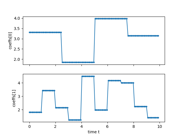
This creates a callable with signature (p, t) that returns p[int(len(p)*t/duration)], such that the passed parameters are the function values for different time bins. Note how the number of time bins is implicitly defined through the length of the parameters. In the following example, we are going to use 4 and 10 time bins defined through the length of parameters, respectively. Let us create uniformly random parameters between 0 and 5 and plot the corresponding piece-wise-constant function sampled at 100 different points in time.

key = jax.random.PRNGKey(777)
subkeys = jax.random.split(key, 2) # creates a list of two sub-keys
theta0 = jax.random.uniform(subkeys[0], shape=[4], maxval=5)
theta1 = jax.random.uniform(subkeys[1], shape=[10], maxval=5)
theta = [theta0, theta1]

ts = jnp.linspace(0.0, timespan, 100)[:-1]
fig, axs = plt.subplots(nrows=2, sharex=True)
for i in range(2):
    ax = axs[i]
    ax.plot(ts, coeffs[i](theta[i], ts), ".-")
    ax.set_ylabel(f"coeffs[{i}]")
ax.set_xlabel("time t")
plt.show()

We can use these callables as before to construct a ParametrizedHamiltonian().

ops = [qml.PauliX(i) for i in range(2)]
H = qml.pulse.ParametrizedHamiltonian(coeffs, ops)
print(H(theta, 0.5))

Out:

(3.31518202727953*(PauliX(wires=[0]))) + (1.817160952485034*(PauliX(wires=[1])))

Note that this construction is equivalent to using qml.dot.

Variational quantum eigensolver with pulse programming

We can now use the ability to access gradients to perform the variational quantum eigensolver on the pulse level (ctrl-VQE) as is done in 1. For a more general introduction to VQE, see A brief overview of VQE. First, we define the molecular Hamiltonian whose energy expectation value we want to minimize. This serves as our objective Hamiltonian. We are using \(\text{HeH}^+\) as a simple example and load it from the PennyLane quantum datasets website. We are going to use the tapered Hamiltonian, which makes use of symmetries to reduce the number of qubits, see Qubit tapering for details.

data = qml.data.load("qchem", molname="HeH+", basis="STO-3G", bondlength=1.5)[0]
H_obj = data.tapered_hamiltonian

# casting the Hamiltonian coefficients to a jax Array
H_obj = qml.Hamiltonian(jnp.array(H_obj.coeffs), H_obj.ops)
E_exact = data.fci_energy
n_wires = len(H_obj.wires)

As a realistic physical system with pulse level control, we are considering a coupled transmon qubit system with the constant drift term Hamiltonian

\[H_D = \sum_q \omega_q a_q^\dagger a_q - \sum_q \frac{\delta_q}{2} a^\dagger_q a^\dagger_q a_q a_q + \sum_{\langle pq \rangle} g_{pq} a^\dagger_p a_q\]

with bosonic creation and annihilation operators. The anharmonicity \(\delta_q\) is describing the contribution to higher energy levels. We are only going to consider the qubit subspace and hence set this term to zero. The order of magnitude of the resonance frequencies \(\omega_q\) and coupling strength \(g_{pq}\) are taken from 1 (in GHz). Let us construct the Hamiltonian in PennyLane:

def a(wires):
    return 0.5 * qml.PauliX(wires) + 0.5j * qml.PauliY(wires)

def ad(wires):
    return 0.5 * qml.PauliX(wires) - 0.5j * qml.PauliY(wires)

omega = 2 * jnp.pi * jnp.array([4.8080, 4.8333])
g = 2 * jnp.pi * jnp.array([0.01831, 0.02131])

H_D = qml.dot(omega, [ad(i) @ a(i) for i in range(n_wires)])
H_D += qml.dot(
    g, [ad(i) @ a((i + 1) % n_wires) + ad((i + 1) % n_wires) @ a(i) for i in range(n_wires)]
)

The system is driven under the control term

\[H_C(t) = \sum_q \Omega_q(t) \left(e^{i\nu_q t} a_q + e^{-i\nu_q t} a^\dagger_q \right)\]

with the (real) time-dependent amplitudes \(\Omega_q(t)\) and frequencies \(\nu_q\) of the drive. We let \(\Omega(t)\) be a real piecewise-constant function whose values are optimized. In a transmon qubit systems, entangling gates such as CNOT are realized by driving a target qubit with the resonance frequency of the control qubit. This is referred to as cross resonance and is described in 2. Here, we allow for more general two-qubit interactions by training the drive frequency \(\nu_q\) on each qubit.

For this drive, there are certain restrictions by the hardware that we want to already account for to make our simulation as realistic as possible. We therefore restrict the amplitude to \(\pm 20 \text{MHz}\) and the frequency deviation \(\Delta \nu_q = \omega_q - \nu_q\) to \(\pm 1 \text{GHz}\) (as is done in 1). We achieve this by normalizing the respective quantities with a shifted sigmoid \(\mathcal{N}(x) = \frac{1 - e^{-x}}{1 + e^{-x}}\), which ensures differentiability.

def normalize(x):
    """Differentiable normalization to +/- 1 outputs (shifted sigmoid)"""
    return (1 - jnp.exp(-x))/(1 + jnp.exp(-x))

# Because ParametrizedHamiltonian expects each callable function to have the signature
# f(p, t) but we have additional parameters it depends on, we create a wrapper function
# that constructs the callables with the appropriate parameters imprinted on them
def drive_field(T, omega, sign=1.0):
    def wrapped(p, t):
        # The first len(p)-1 values of the trainable params p characterize the pwc function
        amp = qml.pulse.pwc(T)(p[:-1], t)
        # The amplitude is normalized to maximally reach +/-20MHz (0.02GHz)
        amp = 0.02*normalize(amp)

        # The last value of the trainable params p provides the drive frequency deviation
        # We normalize as the difference to drive can maximally be +/-1 GHz
        d_angle = normalize(p[-1])
        phase = jnp.exp(sign * 1j * (omega + d_angle) * t)
        return amp * phase

    return wrapped

duration = 15.0

fs = [drive_field(duration, omega[i], 1.0) for i in range(n_wires)]
fs += [drive_field(duration, omega[i], -1.0) for i in range(n_wires)]
ops = [a(i) for i in range(n_wires)]
ops += [ad(i) for i in range(n_wires)]

H_C = qml.dot(fs, ops)

Overall, we end up with the time-dependent parametrized Hamiltonian \(H(p, t) = H_D + H_C(p, t)\) under which the system is evolved for the given time window of 15ns. Note that we are expressing time in nanoseconds (\(10^{-9}\) s) and frequencies (and energies) in gigahertz (\(10^{9}\) Hz), such that both exponents cancel.

H_pulse = H_D + H_C

Now we define the qnode that computes the expectation value of the molecular Hamiltonian.

dev = qml.device("default.qubit.jax", wires=range(n_wires))

@qml.qnode(dev, interface="jax")
def qnode(theta, t=duration):
    qml.BasisState(list(data.tapered_hf_state), wires=H_obj.wires)
    qml.evolve(H_pulse)(params=(*theta, *theta), t=t)
    return qml.expval(H_obj)

value_and_grad = jax.jit(jax.value_and_grad(qnode))

We now have all the ingredients to run our ctrl-VQE program. We use the adam implementation in optax, a package for optimizations in jax.

It has been shown that the loss landscapes of pulse programs are trap-free for a variety of conditions and loss functions, including ours 5. In practice however, we see that the optimization is senstive to the initial values of the parameters and the optimization strategy. In particular, we often find ourselves with very slow progress during optimization, indicating wide flat regions in the loss landscape. This can be salvaged by increasing the learning rate. Sometimes, it proved advantageous to increase the learning rate after an initial finer search for a better starting point. Further, we note that with the increase in the number of parameters due to the continuous evolution, the optimization becomes harder.

Whether or not that is due to the increased parameter search space or an inherent effect of pulse programs like barren plateaus in variational quantum circuits is to be determined in future work.

We systematically tried a variety of combinations of learning rate schedule, optimizer, and initial values. Here, we provide one possible choice leading to good results.

We choose t_bins = 100 segments for the piece-wise-constant parametrization of the pulses.

t_bins = 100  # number of time bins

key = jax.random.PRNGKey(999)
theta = 0.9*jax.random.uniform(key, shape=jnp.array([n_wires, t_bins+1]))

import optax
from datetime import datetime

n_epochs = 60

# The following block creates a constant schedule of the learning rate
# that increases from 0.1 to 0.5 after 10 epochs
schedule0 = optax.constant_schedule(1e-1)
schedule1 = optax.constant_schedule(5e-1)
schedule = optax.join_schedules([schedule0, schedule1], [10])
optimizer = optax.adam(learning_rate=schedule)
opt_state = optimizer.init(theta)

energy = np.zeros(n_epochs + 1)
energy[0] = qnode(theta)
gradients = np.zeros(n_epochs)

## Compile the evaluation and gradient function and report compilation time
time0 = datetime.now()
_ = value_and_grad(theta)
time1 = datetime.now()
print(f"grad and val compilation time: {time1 - time0}")

## Optimization loop
for n in range(n_epochs):
    val, grad_circuit = value_and_grad(theta)
    updates, opt_state = optimizer.update(grad_circuit, opt_state)
    theta = optax.apply_updates(theta, updates)

    energy[n + 1] = val
    gradients[n] = np.mean(np.abs(grad_circuit))

    if not n % 10:
        print(f"{n+1} / {n_epochs}; energy discrepancy: {val-E_exact}")
        print(f"mean grad: {gradients[n]}")

Out:

grad and val compilation time: 0:00:05.038250
1 / 60; energy discrepancy: 0.002643141567067353
mean grad: 6.610892798376223e-05
11 / 60; energy discrepancy: 0.0013625294261405685
mean grad: 7.082381803587231e-06
21 / 60; energy discrepancy: 0.0011910338900049666
mean grad: 1.5285189674744793e-05
31 / 60; energy discrepancy: 0.0008837548164963849
mean grad: 3.8022378252743766e-05
41 / 60; energy discrepancy: 0.0005214781252078637
mean grad: 8.45686025583449e-06
51 / 60; energy discrepancy: 0.0004393137537590519
mean grad: 9.616186119311038e-06

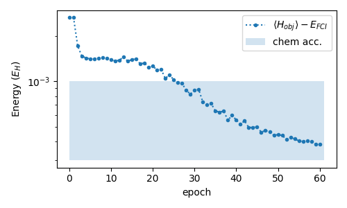
We see that we have converged to chemical accuracy after half the number of epochs.

fig, ax = plt.subplots(nrows=1, figsize=(5, 3), sharex=True)

y = np.array(energy) - E_exact
ax.plot(y, ".:", label="$\\langle H_{{obj}}\\rangle - E_{{FCI}}$")
ax.fill_between([0, len(y)], [1e-3] * 2, 3e-4, alpha=0.2, label="chem acc.")
ax.set_yscale("log")
ax.set_ylabel("Energy ($E_H$)")
ax.set_xlabel("epoch")
ax.legend()

plt.tight_layout()
plt.show()

We can also visualize the envelopes for each qubit in time. We only plot the real amplitude \(\Omega(t)\) and indicate the deviation \(\Delta \nu_q = \omega_q - \nu_q\) of the drive frequency \(\nu_q\) from the qubit frequency \(\omega_q\) in the labels.

n_channels = n_wires
ts = jnp.linspace(0, duration, t_bins)
fig, axs = plt.subplots(nrows=n_channels, figsize=(5, 2 * n_channels), sharex=True)
for n in range(n_channels):
    ax = axs[n]
    label = f"$\\Delta \\nu_{n}$: {normalize(theta[n][-1]):.3}"
    ax.plot(ts, 0.02*normalize(theta[n][:-1]), ".:", label=label)
    ax.set_ylabel(f"$amp_{n}$ (GHz)")
    ax.legend()
ax.set_xlabel("t (ns)")

plt.tight_layout()
plt.show()

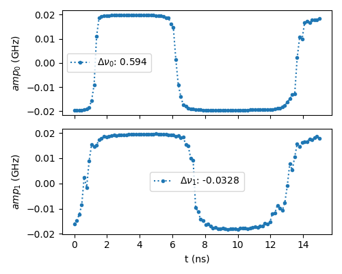
Note that we obtain bang-bang like solutions as indicated in 4, making it likely we are close to the minimal evolution time with 15ns.

Conclusion

Pulse programming is an exciting new field within noisy quantum computing. By skipping the digital abstraction, one can write variational programs on the hardware level, potentially minimizing the computation time. Ideally, this allows for effectively deeper circuits on noisy hardware. On the other hand, the possibility to continuously vary the Hamiltonian interaction in time significantly increases the parameter space. A good parametrization trading off flexibility and the number of parameters is therefore necessary as systems scale up. Further, the increased flexibility also affects the search space in Hilbert space that pulse gates can reach. Barren plateaus in variational quantum algorithms are typically due to a lack of a good inductive bias in the ansatz, i.e. having a search space that is too large. It is therefore crucial to find physically motivated ansätze for pulse programs.

References

1(1,2,3,4)

Oinam Romesh Meitei, Bryan T. Gard, George S. Barron, David P. Pappas, Sophia E. Economou, Edwin Barnes, Nicholas J. Mayhall “Gate-free state preparation for fast variational quantum eigensolver simulations: ctrl-VQE” arXiv:2008.04302, 2020

2(1,2)

Sarah Sheldon, Easwar Magesan, Jerry M. Chow, Jay M. Gambetta “Procedure for systematically tuning up crosstalk in the cross resonance gate” arXiv:1603.04821, 2016.

3

Jiaqi Leng, Yuxiang Peng, Yi-Ling Qiao, Ming Lin, Xiaodi Wu “Differentiable Analog Quantum Computing for Optimization and Control” arXiv:2210.15812, 2022

4

Ayush Asthana, Chenxu Liu, Oinam Romesh Meitei, Sophia E. Economou, Edwin Barnes, Nicholas J. Mayhall “Minimizing state preparation times in pulse-level variational molecular simulations” arXiv:2203.06818, 2022.

5

Benjamin Russell, Herschel Rabitz, Rebing Wu “Quantum Control Landscapes Are Almost Always Trap Free” arXiv:1608.06198, 2016.

About the author

Korbinian Kottmann

Korbinian is a Quantum Scientist at Xanadu, interested in quantum simulation and quantum software.

demos/tutorial_pulse_programming101

 

Download Python script

 

Download Notebook

 

View on GitHub