Note
Click here to download the full example code
Implicit differentiation of variational quantum algorithms
Authors: Shahnawaz Ahmed and Juan Felipe Carrasquilla Álvarez — Posted: 28 November 2022. Last updated: 28 November 2022.
In 1638, René Descartes, intrigued by (then amateur) Pierre de Fermat’s method of computing tangents, challenged Fermat to find the tangent to a complicated curve — now called the folium of Descartes:
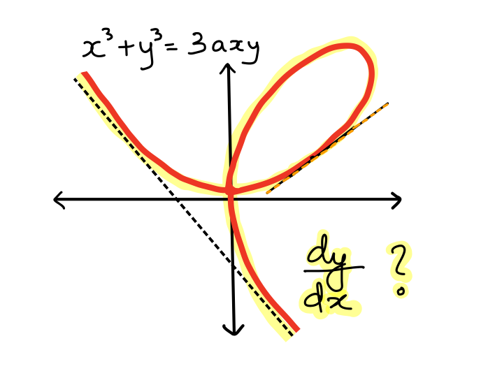
With its cubic terms, this curve represents an implicit equation which cannot be written as a simple expression \(y = f(x)\). Therefore the task of calculating the tangent function seemed formidable for the method Descartes had then, except at the vertex. Fermat successfully provided the tangents at not just the vertex but at any other point on the curve, baffling Descartes and legitimizing the intellectual superiority of Fermat. The technique used by Fermat was implicit differentiation 1. In the above equation, we can begin by take derivatives on both sides and re-arrange the terms to obtain \(dy/dx\).
Implicit differentiation can be used to compute gradients of such functions that cannot be written down explicitly using simple elementary operations. It is a basic technique of calculus that has recently found many applications in machine learning — from hyperparameter optimization to the training of neural ordinary differential equations (ODEs), and it has even led to the definition of a whole new class of architectures, called Deep Equilibrium Models (DEQs) 4.
Introduction
The idea of implicit differentiation can be applied in quantum physics to extend the power of automatic differentiation to situations where we are not able to explicitly write down the solution to a problem. As a concrete example, consider a variational quantum algorithm (VQA) that computes the ground-state solution of a parameterized Hamiltonian \(H(a)\) using a variational ansatz \(|\psi_{z}\rangle\), where \(z\) are the variational parameters. This leads to the solution
As we change \(H(a)\), the solution also changes, but we do not obtain an explicit function for \(z^{*}(a)\). If we are interested in the properties of the solution state, we could measure the expectation values of some operator \(A\) as
With a VQA, we can find a solution to the optimization for a fixed \(H(a)\). However, just like with the folium of Descartes, we do not have an explicit solution, so the gradient \(\partial_a \langle A \rangle (a)\) is not easy to compute. The solution is only implicitly defined.
Automatic differentiation techniques that construct an explicit computational graph and differentiate through it by applying the chain rule for gradient computation cannot be applied here easily. A brute-force application of automatic differentiation that finds \(z^{*}(a)\) throughout the full optimization would require us to keep track of all intermediate variables and steps in the optimization and differentiate through them. This could quickly become computationally expensive and memory-intensive for quantum algorithms. Implicit differentiation provides an alternative way to efficiently compute such a gradient.
Similarly, there exist various other interesting quantities that can be written as gradients of a ground-state solution, e.g., nuclear forces in quantum chemistry, permanent electric dipolestatic polarizability, the static hyperpolarizabilities of various orders, fidelity susceptibilities, and geometric tensors. All such quantities could possibly be computed using implicit differentiation on quantum devices. In our recent work we present a unified way to implement such computations and other applications of implicit differentiation through variational quantum algorithms 2.
In this demo we show how implicit gradients can be computed using a variational algorithm written in PennyLane and powered by a modular implicit differentiation implementation provided by the tool JAXOpt 3. We compute the generalized susceptibility for a spin system by using a variational ansatz to obtain a ground-state and implicitly differentiating through it. In order to compare the implicit solution, we find the exact ground-state through eigendecomposition and determine gradients using automatic differentiation. Even though eigendecomposition may become unfeasible for larger systems, for a small number of spins, it suffices for a comparison with our implicit differentiation approach.
Implicit Differentiation
We consider the differentiation of a solution of the root-finding problem, defined by
A function \(z^{*}(a)\) that satisfies \(f(z^{*}(a), a) = 0\) gives a solution map for fixed values of \(a\). An explicit analytical solution is, however, difficult to obtain in general. This means that the direct differentiation of \(\partial_a z^{*}(a)\) is not always possible. Despite that, some iterative algorithms may be able to compute the solution by starting from an initial set of values for \(z\), e.g., using a fixed-point solver. The optimality condition \(f(z^{*}(a), a) = 0\) tells the solver when a solution is found.
Implicit differentiation can be used to compute \(\partial_a z^{*}(a)\) more efficiently than brute-force automatic differentiation, using only the solution \(z^{*}(a)\) and partial derivatives at the solution point. We do not have to care about how the solution is obtained and, therefore, do not need to differentiate through the solution-finding algorithm 3.
The Implicit function theorem is a statement about how the set of zeros of a system of equations is locally given by the graph of a function under some conditions. It can be extended to the complex domain and we state the theorem (informally) below 6.
Implicit function theorem (IFT) (informal)
If \(f(z, a)\) is some analytic function where in a local neighbourhood around \((z_0, a_0)\) we have \(f(z_0, a_0) = 0\), there exists an analytic solution \(z^{*}(a)\) that satisfies \(f(z^{*}(a), a) = 0\).
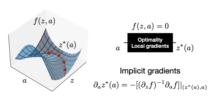
In the figure above we can see solutions to the optimality condition \(f(z, a) = 0 \). According to the IFT, the solution function is analytic, which means it can be differentiated at the solution points by simply differentiating the above equation with respect to \(a\), as
which leads to
This shows that implicit differentiation can be used in situations where we can phrase our optimization problem in terms of an optimality condition or a fixed point equation that can be solved. In case of optimization tasks, such an optimality condition would be that, at the minima, the gradient of the cost function is zero — i.e.,
Then, as long as we have the solution, \(z^{*}(a)\), and the partial derivatives at the solution (in this case the Hessian of the cost function \(g(z, a)\)), \((\partial_a f, \partial_z f)\), we can compute implicit gradients. Note that, for a multivariate function, the inversion \((\partial_{z} f(z_0, a_0) )^{-1}\) needs to be defined and easy to compute. It is possible to approximate this inversion in a clever way by constructing a linear problem that can be solved approximately 3, 4.
Implicit differentiation through a variational quantum algorithm
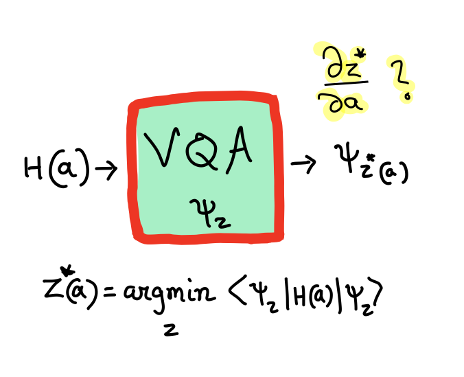
We now discuss how the idea of implicit differentiation can be applied to variational quantum algorithms. Let us take a parameterized Hamiltonian \(H(a)\), where \(a\) is a parameter that can be continuously varied. If \(|\psi_{z}\rangle\) is a variational solution to the ground state of \(H(a)\), then we can find a \(z^*(a)\) that minimizes the ground state energy, i.e.,
where \(E(z, a)\) is the energy function. We consider the following Hamiltonian
where \(J\) is the interaction, \(\sigma^{x}\) and \(\sigma^{z}\) are the spin-\(\frac{1}{2}\) operators and \(\gamma\) is the magnetic field strength (which is taken to be the same for all spins). The term \(A = \frac{1}{N}\sum_i \sigma^{z}_i\) is the magnetization and a small non-zero magnetization \(\delta\) is added for numerical stability. We have assumed a circular chain such that in the interaction term the last spin (\(i = N-1\)) interacts with the first (\(i=0\)).
Now we could find the ground state of this Hamiltonian by simply taking the eigendecomposition and applying automatic differentiation through the eigendecomposition to compute gradients. We will compare this exact computation for a small system to the gradients given by implicit differentiation through a variationally obtained solution.
We define the following optimality condition at the solution point:
In addition, if the conditions of the implicit function theorem are also satisfied, i.e., \(f\) is continuously differentiable with a non-singular Jacobian at the solution, then we can apply the chain rule and determine the implicit gradients easily.
At this stage, any other complicated function that depends on the variational ground state can be easily differentiated using automatic differentiation by plugging in the value of \(partial_a z^{*}(a)\) where it is required. The expectation value of the operator \(A\) for the ground state is
In the case where \(A\) is just the energy, i.e., \(A = H(a)\), the Hellmann–Feynman theorem allows us to easily compute the gradient. However, for a general operator we need the gradients \(\partial_a z^{*}(a)\), which means that implicit differentiation is a very elegant way to go beyond the Hellmann–Feynman theorem for arbitrary expectation values.
Let us now dive into the code and implementation.
Talk is cheap. Show me the code. - Linus Torvalds
Implicit differentiation of ground states in PennyLane
from functools import reduce

from operator import add

import jax
from jax import jit
import jax.numpy as jnp
from jax.config import config

import pennylane as qml
import numpy as np

import jaxopt

import matplotlib.pyplot as plt

jax.config.update('jax_platform_name', 'cpu')

# Use double precision numbers
config.update("jax_enable_x64", True)
Defining the Hamiltonian and measurement operator
We define the Hamiltonian by building the non-parametric part separately and adding the parametric part to it as a separate term for efficiency. Note that, for the example of generalized susceptibility, we are measuring expectation values of the operator \(A\) that also defines the parametric part of the Hamiltonian. However, this is not necessary and we could compute gradients for any other operator using implicit differentiation, as we have access to the gradients \(\partial_a z^{*}(a)\).
N = 4
J = 1.0
gamma = 1.0

def build_H0(N, J, gamma):
    """Builds the non-parametric part of the Hamiltonian of a spin system.

    Args:
        N (int): Number of qubits/spins.
        J (float): Interaction strength.
        gamma (float): Interaction strength.

    Returns:
        qml.Hamiltonian: The Hamiltonian of the system.
    """
    H = qml.Hamiltonian([], [])

    for i in range(N - 1):
        H += -J * qml.PauliZ(i) @ qml.PauliZ(i + 1)

    H += -J * qml.PauliZ(N - 1) @ qml.PauliZ(0)

    # Transverse
    for i in range(N):
        H += -gamma * qml.PauliX(i)

    # Small magnetization for numerical stability
    for i in range(N):
        H += -1e-1 * qml.PauliZ(i)

    return H

H0 = build_H0(N, J, gamma)
H0_matrix = qml.matrix(H0)
A = reduce(add, ((1 / N) * qml.PauliZ(i) for i in range(N)))
A_matrix = qml.matrix(A)
Computing the exact ground state through eigendecomposition
We now define a function that computes the exact ground state using eigendecomposition. Ideally, we would like to take gradients of this function. It is possible to simply apply automatic differentiation through this exact ground-state computation. JAX has an implementation of differentiation through eigendecomposition.
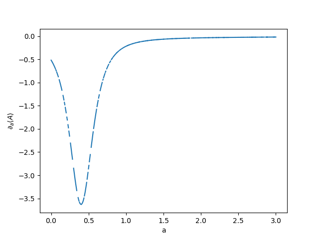
Note that we have some points in this plot that are nan, where the gradient
computation through the eigendecomposition does not work. We will see later that
the computation through the VQA is more stable.
@jit
def ground_state_solution_map_exact(a: float) -> jnp.array:
    """The ground state solution map that we want to differentiate
    through, computed from an eigendecomposition.

    Args:
        a (float): The parameter in the Hamiltonian, H(a).

    Returns:
        jnp.array: The ground state solution for the H(a).
    """
    H = H0_matrix + a * A_matrix
    eval, eigenstates = jnp.linalg.eigh(H)
    z_star = eigenstates[:, 0]
    return z_star


a = jnp.array(np.random.uniform(0, 1.0))
z_star_exact = ground_state_solution_map_exact(a)
Susceptibility computation through the ground state solution map
Let us now compute the susceptibility function by taking gradients of the expectation value of our operator \(A\) w.r.t a. We can use jax.vmap to vectorize the computation over different values of a.
@jit
def expval_A_exact(a):
    """Expectation value of ``A`` as a function of ``a`` where we use the
    ``ground_state_solution_map_exact`` function to find the ground state.

    Args:
        a (float): The parameter defining the Hamiltonian, H(a).

    Returns:
        float: The expectation value of A calculated using the variational state
               that should be the ground state of H(a).
    """
    z_star = ground_state_solution_map_exact(a)
    eval = jnp.conj(z_star.T) @ A_matrix @ z_star
    return eval.real

# the susceptibility is the gradient of the expectation value
_susceptibility_exact = jax.grad(expval_A_exact)
susceptibility_exact = jax.vmap(_susceptibility_exact)

alist = jnp.linspace(0, 3, 1000)
susvals_exact = susceptibility_exact(alist)

plt.plot(alist, susvals_exact)
plt.xlabel("a")
plt.ylabel(r"$\partial_{a}\langle A \rangle$")
plt.show()
Computing susceptibility through implicit differentiation
We use PennyLane to find a variational ground state for the Hamiltonian
\(H(a)\) and compute implicit gradients through the variational
optimization procedure. We use the jaxopt library which contains an
implementation of gradient descent that automatically comes with implicit
differentiation capabilities. We are going to use that to obtain
susceptibility by taking gradients through the ground-state minimization.
Defining the variational state
In PennyLane, we can implement a variational state in different ways, by
defining a quantum circuit. There are also useful template circuits available, such as
SimplifiedTwoDesign, which implements the two-design ansatz.
The ansatz consists of layers of Pauli-Y rotations with
controlled-Z gates. In each layer there are N - 1 parameters for the Pauli-Y gates.
Therefore, the ansatz is efficient as long as we have enough layers for it
so that is expressive enough to represent the ground-state.
We set n_layers = 5, but you can redo this example with fewer layers to see
how a less expressive ansatz leads to error in the susceptibility computation.
Note
The setting shots=None makes for the computation of gradients using reverse-mode
autodifferentiation (backpropagation). It allows us to just-in-time (JIT)
compile the functions that compute expectation values and gradients.
In a real device we would use a finite number of shots and the gradients would be computed
using the parameter-shift rule. However, this may be slower.
variational_ansatz = qml.SimplifiedTwoDesign
n_layers = 5
weights_shape = variational_ansatz.shape(n_layers, N)

dev = qml.device("default.qubit.jax", wires=N, shots=None)

@jax.jit
@qml.qnode(dev, interface="jax")
def energy(z, a):
    """Computes the energy for a Hamiltonian H(a) using a measurement on the
    variational state U(z)|0> with U(z) being any circuit ansatz.

    Args:
        z (jnp.array): The variational parameters for the ansatz (circuit)
        a (jnp.array): The Hamiltonian parameters.

    Returns:
        float: The expectation value (energy).
    """
    variational_ansatz(*z, wires=range(N))
    # here we compute the Hamiltonian coefficients and operations
    # 'by hand' because the qml.Hamiltonian class does not support
    # operator arithmetic with JAX device arrays.
    coeffs = jnp.concatenate([H0.coeffs, a * A.coeffs])
    return qml.expval(qml.Hamiltonian(coeffs, H0.ops + A.ops))


z_init = [jnp.array(2 * np.pi * np.random.random(s)) for s in weights_shape]
a = jnp.array([0.5])
print("Energy", energy(z_init, a))
Out:
Energy -0.07922925936304472
Computing ground states using a variational quantum algorithm (VQA)
We construct a loss function that defines a ground-state minimization
task. We are looking for variational parameters z that minimize the energy
function. Once we find a set of parameters z, we wish to compute the
gradient of any function of the ground state w.r.t. a.
For the implicit differentiation we will use the tool jaxopt, which implements
modular implicit differentiation for various cases; e.g., for fixed-point
functions or optimization. We can directly use jaxopt to optimize our loss
function and then compute implicit gradients through it.
It all works due to PennyLane’s integration with JAX.
The implicit differentiation formulas can even be implemented manually with JAX.
These formulas are implemented in a modular way, using the
jaxopt.GradientDescent optimizer with implicit_diff=True.
We use the seamless integration between PennyLane, JAX
and JAXOpt to compute the susceptibility.
Since everything is written in JAX, simply calling the
jax.grad function works as jaxopt computes the implicit gradients and
plugs it any computation used by jax.grad. We can also just-in-time (JIT)
compile all functions although the compilation may take some time as the
number of spins or variational ansatz becomes more complicated. Once compiled,
all computes run very fast for any parameters.
def ground_state_solution_map_variational(a, z_init):
    """The ground state solution map that we want to differentiate
    through.

    Args:
        a (float): The parameter in the Hamiltonian, H(a).
        z_init [jnp.array(jnp.float)]: The initial guess for the variational
                                       parameters.

    Returns:
        z_star (jnp.array [jnp.float]): The parameters that define the
                                        ground-state solution.
    """
    @jax.jit
    def loss(z, a):
        """Loss function for the ground-state minimization with regularization.

        Args:
            z (jnp.array): The variational parameters for the ansatz (circuit)
            a (jnp.array): The Hamiltonian parameters.

        Returns:
            float: The loss value (energy + regularization)
        """
        return (
            energy(z, a) + 0.001 * jnp.sum(jnp.abs(z[0])) + 0.001 * jnp.sum(jnp.abs(z[1]))
        )
    gd = jaxopt.GradientDescent(
        fun=loss,
        stepsize=1e-2,
        acceleration=True,
        maxiter=1000,
        implicit_diff=True,
        tol=1e-15,
    )
    z_star = gd.run(z_init, a=a).params
    return z_star

a = jnp.array(np.random.uniform(0, 1.0))  # A random ``a``
z_star_variational = ground_state_solution_map_variational(a, z_init)
Computing gradients through the VQA simply by calling jax.grad
We can compute the susceptibility values by simply using jax.grad. After the
first call, the function is compiled and subsequent calls become
much faster.
@jax.jit
@qml.qnode(dev, interface="jax")
def expval_A_variational(z: float) -> float:
    """Expectation value of $A$ as a function of $a$ where we use the
    a variational ground state solution map.

    Args:
        a (float): The parameter in the Hamiltonian, H(a).

    Returns:
        float: The expectation value of M on the ground state of H(a)
    """
    variational_ansatz(*z, wires=range(N))
    return qml.expval(A)

@jax.jit
def groundstate_expval_variational(a, z_init) -> float:
    """Computes ground state and calculates the expectation value of the operator M.

    Args:
        a (float): The parameter in the Hamiltonian, H(a).
        z_init [jnp.array(jnp.float)]: The initial guess for the variational parameters.
        H0 (qml.Hamiltonian): The static part of the Hamiltonian
    """
    z_star = ground_state_solution_map_variational(a, z_init)
    return expval_A_variational(z_star)

susceptibility_variational = jax.jit(jax.grad(groundstate_expval_variational, argnums=0))
z_init = [jnp.array(2 * np.pi * np.random.random(s)) for s in weights_shape]
print("Susceptibility", susceptibility_variational(alist[0], z_init))

susvals_variational = []

for i in range(len(alist)):
    susvals_variational.append(susceptibility_variational(alist[i], z_init))

plt.plot(alist, susvals_variational, label="Implicit diff through VQA")
plt.plot(alist, susvals_exact, "--", c="k", label="Automatic diff through eigendecomposition")
plt.xlabel("a")
plt.ylabel(r"$\partial_{a}\langle A \rangle$")
plt.legend()
plt.show()
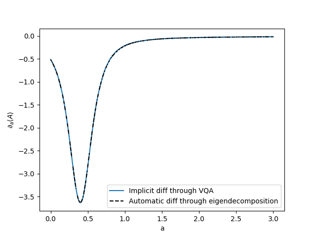
Out:
Susceptibility -0.5126961248004934
PennyLane version and details
print(qml.about())
Out:
Name: PennyLane
Version: 0.30.0
Summary: PennyLane is a Python quantum machine learning library by Xanadu Inc.
Home-page: https://github.com/XanaduAI/pennylane
Author:
Author-email:
License: Apache License 2.0
Location: /home/runner/work/qml/qml/venv/lib/python3.9/site-packages
Requires: appdirs, autograd, autoray, cachetools, networkx, numpy, pennylane-lightning, requests, rustworkx, scipy, semantic-version, toml
Required-by: PennyLane-Cirq, PennyLane-Lightning, PennyLane-qiskit, pennylane-qulacs

Platform info:           Linux-5.15.0-1038-azure-x86_64-with-glibc2.35
Python version:          3.9.16
Numpy version:           1.23.5
Scipy version:           1.10.1
Installed devices:
- lightning.qubit (PennyLane-Lightning-0.31.0.dev5)
- qiskit.aer (PennyLane-qiskit-0.30.1)
- qiskit.basicaer (PennyLane-qiskit-0.30.1)
- qiskit.ibmq (PennyLane-qiskit-0.30.1)
- qiskit.ibmq.circuit_runner (PennyLane-qiskit-0.30.1)
- qiskit.ibmq.sampler (PennyLane-qiskit-0.30.1)
- default.gaussian (PennyLane-0.30.0)
- default.mixed (PennyLane-0.30.0)
- default.qubit (PennyLane-0.30.0)
- default.qubit.autograd (PennyLane-0.30.0)
- default.qubit.jax (PennyLane-0.30.0)
- default.qubit.tf (PennyLane-0.30.0)
- default.qubit.torch (PennyLane-0.30.0)
- default.qutrit (PennyLane-0.30.0)
- null.qubit (PennyLane-0.30.0)
- qulacs.simulator (pennylane-qulacs-0.29.0)
- cirq.mixedsimulator (PennyLane-Cirq-0.29.0)
- cirq.pasqal (PennyLane-Cirq-0.29.0)
- cirq.qsim (PennyLane-Cirq-0.29.0)
- cirq.qsimh (PennyLane-Cirq-0.29.0)
- cirq.simulator (PennyLane-Cirq-0.29.0)
None
Conclusion
We have shown how a combination of JAX, PennyLane and JAXOpt can be used to compute implicit gradients through a VQA. The ability to compute such gradients opens up new possibilities, e.g., the design of a Hamiltonian such that its ground-state has certain properties. It is also possible to perhaps look at this inverse-design of the Hamiltonian as a control problem. Implicit differentiation in the classical setting allows defining a new type of neural network layer — implicit layers such as neural ODEs. In a similar way, we hope this demo the inspires creation of new architectures for quantum neural networks, perhaps a quantum version of neural ODEs or quantum implicit layers.
In future works, it would be important to assess the cost of running implicit differentiation through an actual quantum computer and determine the quality of such gradients as a function of noise as explored in a related recent work 5.
References
- 1
Jaume Paradís, Josep Pla & Pelegrí Viader “Fermat and the Quadrature of the Folium of Descartes” The American Mathematical Monthly, 111:3, 216-229 10.1080/00029890.2004.11920067, 2004.
- 2
Shahnawaz Ahmed, Nathan Killoran, Juan Felipe Carrasquilla Álvarez “Implicit differentiation of variational quantum algorithms arXiv:2211.13765, 2022.
- 3(1,2,3)
Mathieu Blondel, Quentin Berthet, Marco Cuturi, Roy Frostig, Stephan Hoyer, Felipe Llinares-López, Fabian Pedregosa, Jean-Philippe Vert “Efficient and modular implicit differentiation” arXiv:2105.15183, 2021.
- 4(1,2)
Zico Kolter, David Duvenaud, Matt Johnson. “Deep Implicit Layers - Neural ODEs, Deep Equilibirum Models, and Beyond” http://implicit-layers-tutorial.org, 2021.
- 5
Olivia Di Matteo, R. M. Woloshyn “Quantum computing fidelity susceptibility using automatic differentiation” arXiv:2207.06526, 2022.
- 6
Chang, Hung-Chieh, Wei He, and Nagabhushana Prabhu. “The analytic domain in the implicit function theorem.” JIPAM. J. Inequal. Pure Appl. Math 4.1, (2003).
About the authors

Shahnawaz Ahmed

Juan Felipe Carrasquilla Alvarez
Total running time of the script: ( 4 minutes 22.686 seconds)