Classically-Boosted Variational Quantum Eigensolver

Authors: Joana Fraxanet & Isidor Schoch (Xanadu Residents). Posted: 31 October 2022. Last updated: 31 October 2022.

One of the most important applications of quantum computers is expected to be the computation of ground-state energies of complicated molecules and materials. Even though there are already some solid proposals on how to tackle these problems when fault-tolerant quantum computation comes into play, we currently live in the noisy intermediate-scale quantum (NISQ) era, meaning that we can only access noisy and limited devices. That is why a large part of the current research on quantum algorithms is focusing on what can be done with few resources. In particular, most proposals rely on variational quantum algorithms (VQA), which are optimized classically and adapt to the limitations of the quantum devices. For the specific problem of computing ground-state energies, the paradigmatic algorithm is the Variational Quantum Eigensolver (VQE) algorithm.

Although VQE is intended to run on NISQ devices, it is nonetheless sensitive to noise. This is particularly problematic when applying VQE to complicated molecules which requires a large number of gates. As a consequence, several modifications to the original VQE algorithm have been proposed. These variants are usually intended to improve the algorithm’s performance on NISQ-era devices.

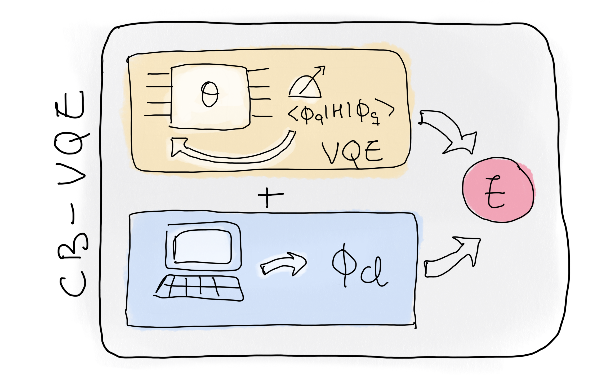
In this demo, we will go through one of these proposals step-by-step: the Classically-Boosted Variational Quantum Eigensolver (CB-VQE) 1. Implementing CB-VQE reduces the number of measurements required to obtain the ground-state energy with a certain precision. This is done by making use of classical states, which in this context are product states that can be written as a single Slater determinant and that already contain some information about the ground-state of the problem. Their structure allows for efficient classical computation of expectation values. An example of such classical state would be the Hartree-Fock state, in which the electrons occupy the molecular orbitals with the lowest energy.

We will restrict ourselves to the \(H_2\) molecule for the sake of simplicity. First, we will give a short introduction to how to perform standard VQE for the molecule of interest. For more details, we recommend the tutorial A brief overview of VQE to learn how to implement VQE for molecules step by step. Then, we will implement the CB-VQE algorithm for the specific case in which we rely only on one classical state⁠—that being the Hartree-Fock state. Finally, we will discuss the number of measurements needed to obtain a certain error-threshold by comparing the two methods.

Let’s get started!

Prerequisites: Standard VQE

If you are not already familiar with the VQE family of algorithms and wish to see how one can apply it to the \(H_2\) molecule, feel free to work through the aforementioned demo before reading this section. Here, we will only briefly review the main idea behind standard VQE and highlight the important concepts in connection with CB-VQE.

Given a Hamiltonian \(H\), the main goal of VQE is to find the ground state energy of a system governed by the Schrödinger equation

\[H \vert \phi \rangle = E \vert \phi \rangle.\]

This corresponds to the problem of diagonalizing the Hamiltonian and finding the smallest eigenvalue. Alternatively, one can formulate the problem using the variational principle, in which we are interested in minimizing the energy

\[E = \langle \phi \vert H \vert \phi \rangle.\]

In VQE, we prepare a statevector \(\vert \phi \rangle\) by applying the parameterized ansatz \(A(\Theta)\), represented by a unitary matrix, to an initial state \(\vert 0 \rangle^{\otimes n}\) where \(n\) is the number of qubits. Then, the parameters \(\Theta\) are optimized to minimize a cost function, which in this case is the energy:

\[E(\Theta) = \langle 0 \vert^{\otimes n} A(\Theta)^{\dagger} H A(\Theta) \vert 0 \rangle^{\otimes n}.\]

This is done using a classical optimization method, which is typically gradient descent.

To implement our example of VQE, we first define the molecular Hamiltonian for the \(H_2\) molecule in the minimal STO-3G basis using PennyLane

import pennylane as qml
from pennylane import qchem
from pennylane import numpy as np

symbols = ["H", "H"]
coordinates = np.array([0.0, 0.0, -0.6614, 0.0, 0.0, 0.6614])
basis_set = "sto-3g"
electrons = 2

H, qubits = qchem.molecular_hamiltonian(
    symbols,
    coordinates,
    basis=basis_set,
)

We then initialize the Hartree-Fock state \(\vert \phi_{HF}\rangle=\vert 1100 \rangle\)

hf = qchem.hf_state(electrons, qubits)

Next, we implement the ansatz \(A(\Theta)\). In this case, we use the class AllSinglesDoubles, which enables us to apply all possible combinations of single and double excitations obeying the Pauli principle to the Hartree-Fock state. Single and double excitation gates, denoted \(G^{(1)}(\Theta)\) and \(G^{(2)}(\Theta)\) respectively, are conveniently implemented in PennyLane with SingleExcitation and DoubleExcitation classes. You can find more information about how these gates work in this video and in the demo Givens rotations for quantum chemistry.

singles, doubles = qchem.excitations(electrons=electrons, orbitals=qubits)
num_theta = len(singles) + len(doubles)


def circuit_VQE(theta, wires):
    qml.AllSinglesDoubles(weights=theta, wires=wires, hf_state=hf, singles=singles, doubles=doubles)

Once this is defined, we can run the VQE algorithm. We first need to define a circuit for the cost function.

dev = qml.device("default.qubit", wires=qubits)


@qml.qnode(dev, interface="autograd")
def cost_fn(theta):
    circuit_VQE(theta, range(qubits))
    return qml.expval(H)

We then fix the classical optimization parameters stepsize and max_iteration:

stepsize = 0.4
max_iterations = 30
opt = qml.GradientDescentOptimizer(stepsize=stepsize)
theta = np.zeros(num_theta, requires_grad=True)

Finally, we run the algorithm.

for n in range(max_iterations):
    theta, prev_energy = opt.step_and_cost(cost_fn, theta)
    samples = cost_fn(theta)

energy_VQE = cost_fn(theta)
theta_opt = theta

print("VQE energy: %.4f" % (energy_VQE))
print("Optimal parameters:", theta_opt)

Out:

VQE energy: -1.1362
Optimal parameters: [0.         0.         0.20973221]

Note that as an output we obtain the VQE approximation to the ground state energy and a set of optimized parameters \(\Theta\) that define the ground state through the ansatz \(A(\Theta)\). We will need to save these two quantities, as they are necessary to implement CB-VQE in the following steps.

Classically-Boosted VQE

Now we are ready to present the classically-boosted version of VQE.

The key of this new method relies on the notion of the generalized eigenvalue problem. The main idea is to restrict the problem of finding the ground state to an eigenvalue problem in a subspace \(\mathcal{H}^{\prime}\) of the complete Hilbert space \(\mathcal{H}\). If this subspace is spanned by a combination of both classical and quantum states, we can run parts of our algorithm on classical hardware and thus reduce the number of measurements needed to reach a certain precision threshold. The generalized eigenvalue problem is expressed as

\[\bar{H} \vec{v}= \lambda \bar{S} \vec{v},\]

where the matrix \(\bar{S}\) contains the overlaps between the basis states and \(\bar{H}\) is the Hamiltonian \(H\) projected into the subspace of interest, i.e. with the entries

\[\bar{H}_{\alpha, \beta} = \langle \phi_\alpha \vert H \vert \phi_\beta \rangle,\]

for all \(\vert \phi_\alpha \rangle\) and \(\vert \phi_\beta \rangle\) in \(\mathcal{H}^{\prime}\). For a complete orthonormal basis, the overlap matrix \(\bar{S}\) would simply be the identity matrix. However, we need to take a more general approach which works for a subspace spanned by potentially non-orthogonal states. We can retrieve the representation of \(S\) by calculating

\[\bar{S}_{\alpha, \beta} = \langle \phi_\alpha \vert \phi_\beta \rangle,\]

for all \(\vert \phi_\alpha \rangle\) and \(\vert \phi_\beta \rangle\) in \(\mathcal{H}^{\prime}\). Finally, note that \(\vec{v}\) and \(\lambda\) are the eigenvectors and eigenvalues respectively. Our goal is to find the lowest eigenvalue \(\lambda_0.\)

Equipped with the useful mathematical description of generalized eigenvalue problems, we can now choose our subspace such that some of the states \(\vert \phi_{\alpha} \rangle \in \mathcal{H}^{\prime}\) are classically tractable.

We will consider the simplest case in which the subspace is spanned only by one classical state \(\vert \phi_{HF} \rangle\) and one quantum state \(\vert \phi_{q} \rangle\). More precisely, we define the classical state to be a single Slater determinant, which directly hints towards using the Hartree-Fock state for several reasons. First of all, it is well-known that the Hartree-Fock state is a good candidate to approximate the ground state in the mean-field limit. Secondly, we already computed it when we built the molecular Hamiltonian for the standard VQE!

To summarize, our goal is to build the Hamiltonian \(\bar{H}\) and the overlap matrix \(\bar{S}\), which act on the subspace \(\mathcal{H}^{\prime} \subseteq \mathcal{H}\) spanned by \(\{\vert \phi_{HF} \rangle, \vert \phi_q \rangle\}\). These will be two-dimensional matrices, and in the following sections we will show how to compute all their entries step by step.

As done previously, we start by importing PennyLane, Qchem and differentiable NumPy followed by defining the molecular Hamiltonian in the Hartree-Fock basis for \(H_2\).

symbols = ["H", "H"]
coordinates = np.array([0.0, 0.0, -0.6614, 0.0, 0.0, 0.6614])
basis_set = "sto-3g"

H, qubits = qchem.molecular_hamiltonian(
    symbols,
    coordinates,
    basis=basis_set,
)

Computing Classical Quantities

We first set out to calculate the purely classical part of the Hamiltonian \(H\). Since we only have one classical state this will already correspond to a scalar energy value. The terms can be expressed as

\[H_{11} = \langle \phi_{HF} \vert H \vert \phi_{HF} \rangle \quad \text{and} \quad S_{11} = \langle \phi_{HF} \vert \phi_{HF} \rangle\]

which is tractable using classical methods. This energy corresponds to the Hartree-Fock energy due to our convenient choice of the classical state. Note that the computation of the classical component of the overlap matrix \(S_{11} = \langle \phi_{HF} \vert \phi_{HF} \rangle = 1\) is trivial.

Using PennyLane, we can access the Hartree-Fock energy by looking at the fermionic Hamiltonian, which is the Hamiltonian on the basis of Slater determinants. The basis is organized in lexicographic order, meaning that if we want the entry corresponding to the Hartree-Fock determinant \(\vert 1100 \rangle\), we will have to take the entry \(H_{i,i}\), where \(1100\) is the binary representation of the index \(i\).

hf_state = qchem.hf_state(electrons, qubits)
fermionic_Hamiltonian = H.sparse_matrix().todense()

# we first convert the HF slater determinant to a string
binary_string = "".join([str(i) for i in hf_state])
# we then obtain the integer corresponding to its binary representation
idx0 = int(binary_string, 2)
# finally we access the entry that corresponds to the HF energy
H11 = fermionic_Hamiltonian[idx0, idx0]
S11 = 1

Computing Quantum Quantities

We now move on to the purely quantum part of the Hamiltonian, i.e. the entry

\[H_{22} = \langle \phi_{q} \vert H \vert \phi_{q} \rangle,\]

where \(\vert \phi_q \rangle\) is the quantum state. This state is just the output of the standard VQE with a given ansatz, following the steps in the first section. Therefore, the entry \(H_{22}\) just corresponds to the final energy of the VQE. In particular, note that the quantum state can be written as \(\vert \phi_{q} \rangle = A(\Theta^*) \vert \phi_{HF} \rangle\) where \(A(\Theta^*)\) is the ansatz of the VQE with the optimised parameters \(\Theta^*\). Once again, we have \(S_{22}=\langle \phi_{q} \vert \phi_{q} \rangle = 1\) for the overlap matrix.

H22 = energy_VQE
S22 = 1

Computing Mixed Quantities

The final part of the algorithm computes the cross-terms between the classical and quantum state

\[H_{12} = \langle \phi_{HF} \vert H \vert \phi_{q} \rangle = H_{21}^{\dagger}.\]

This part of the algorithm is slightly more complicated than the previous steps, since we still want to make use of the classical component of the problem in order to minimize the number of required measurements.

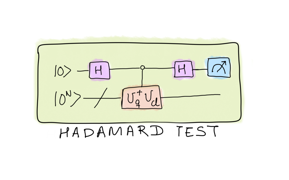
Keep in mind that most algorithms usually perform computations either on fully classically or quantum tractable Hilbert spaces. CB-VQE takes advantage of the classical part of the problem while still calculating a classically-intractable quantity by using the so-called Hadamard test to construct \(H_{12}\). The Hadamard test is a prime example of an indirect measurement, which allows us to measure properties of a state without (completely) destroying it.

As the Hadamard test returns the real part of a coefficient from a unitary representing an operation, we will focus on calculating the quantities

\[H_{12} = \sum_{i} Re(\langle \phi_q \vert i \rangle) \langle i \vert H \vert \phi_{HF} \rangle,\]

\[S_{12} = Re(\langle \phi_q \vert \phi_{HF} \rangle),\]

where \(\lvert i \rangle\) are the computational basis states of the system, i.e. the basis of single Slater determinants. Note that we have to decompose the Hamiltonian into a sum of unitaries. For the problem under consideration, the set of relevant computational basis states for which \(\langle i \vert H \vert \phi_{HF}\rangle \neq 0\) contains all the single and double excitations (allowed by spin symmetries), namely, the states

\[\vert 1100 \rangle, \vert 1001 \rangle, \vert 0110 \rangle, \vert 0011 \rangle.\]

Specifically, the set of computational basis states includes the Hartree-Fock state \(\lvert i_0 \rangle = \vert \phi_{HF} \rangle = \vert 1100 \rangle\) and the projections \(\langle i \vert H \vert \phi_{HF} \rangle\) can be extracted analytically from the fermionic Hamiltonian that we computed above. This is done by accessing the entries by the index given by the binary expression of each Slater determinant.

The Hadamard test is required to compute the real part of \(\langle \phi_q \vert i \rangle\).

To implement the Hadamard test, we need a register of \(n\) qubits given by the size of the molecular Hamiltonian (\(n=4\) in our case) initialized in the state \(\rvert 0 \rangle^{\otimes n}\) and an ancillary qubit prepared in the \(\rvert 0 \rangle\) state.

In order to generate \(\langle \phi_q \vert i \rangle\), we take \(U_q\) such that \(U_q \vert 0 \rangle^{\otimes n} = \vert \phi_q \rangle\). This is equivalent to using the standard VQE ansatz with the optimized parameters \(\Theta^*\) that we obtained in the previous section \(U_q = A(\Theta^*)\). Moreover, we also need \(U_i\) such that \(U_i \vert 0^n \rangle = \vert \phi_i \rangle\). In this case, this is just a mapping of a classical basis state into the circuit consisting of \(X\) gates and can be easily implemented using PennyLane’s function qml.BasisState(i, n)).

wires = range(qubits + 1)
dev = qml.device("default.qubit", wires=wires)


@qml.qnode(dev, interface="autograd")
def hadamard_test(Uq, Ucl, component="real"):
    if component == "imag":
        qml.RX(math.pi / 2, wires=wires[1:])

    qml.Hadamard(wires=[0])
    qml.ControlledQubitUnitary(Uq.conjugate().T @ Ucl, control_wires=[0], wires=wires[1:])
    qml.Hadamard(wires=[0])

    return qml.probs(wires=[0])

Now, we are ready to compute the Hamiltonian cross-terms.

def circuit_product_state(state):
    qml.BasisState(state, range(qubits))


Uq = qml.matrix(circuit_VQE)(theta_opt, range(qubits))

H12 = 0
relevant_basis_states = np.array(
    [[1, 1, 0, 0], [0, 1, 1, 0], [1, 0, 0, 1], [0, 0, 1, 1]], requires_grad=True
)
for j, basis_state in enumerate(relevant_basis_states):
    Ucl = qml.matrix(circuit_product_state)(basis_state)
    probs = hadamard_test(Uq, Ucl)
    # The projection Re(<phi_q|i>) corresponds to 2p-1
    y = 2 * probs[0] - 1
    # We retrieve the quantities <i|H|HF> from the fermionic Hamiltonian
    binary_string = "".join([str(coeff) for coeff in basis_state])
    idx = int(binary_string, 2)
    overlap_H = fermionic_Hamiltonian[idx0, idx]
    # We sum over all computational basis states
    H12 += y * overlap_H
    # y0 corresponds to Re(<phi_q|HF>)
    if j == 0:
        y0 = y

H21 = np.conjugate(H12)

The cross terms of the \(S\) matrix are defined making use of the projections with the Hartree-Fock state.

S12 = y0
S21 = y0.conjugate()

Solving the generalized eigenvalue problem

We are ready to solve the generalized eigenvalue problem. For this, we will build the matrices \(H\) and \(S\) and use scipy to obtain the lowest eigenvalue.

from scipy import linalg

S = np.array([[S11, S12], [S21, S22]])
H = np.array([[H11, H12], [H21, H22]])

evals = linalg.eigvals(H, S)
energy_CBVQE = np.min(evals).real

print("CB-VQE energy %.4f" % (energy_CBVQE))

Out:

CB-VQE energy -1.1362

Measurement analysis

CB-VQE is helpful when it comes to reducing the number of measurements that are required to reach a given precision in the ground state energy. In fact, for very small systems it can be shown that the classically-boosted method reduces the number of required measurements by a factor of \(1000\) 1.

Let’s see if this is the case for the example above. Now that we know how to run standard VQE and CB-VQE algorithms, we can re-run the code above for a finite number of measurements. This is done by specifying the number of shots in the definition of the devices, for example, num_shots = 20. By doing this, Pennylane will output the expectation value of the energy computed from a sample of 20 measurements. Then, we simply run both VQE and CB-VQE enough times to obtain statistics on the results.

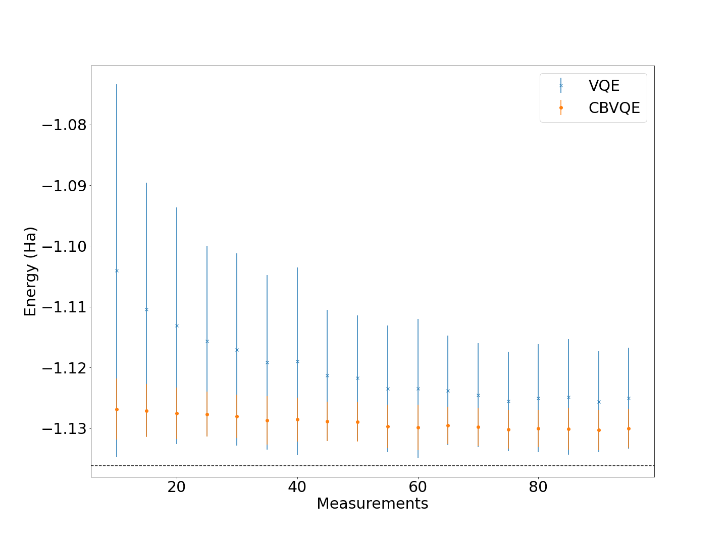
In the plot above, the dashed line corresponds to the true ground state energy of the \(H_2\) molecule. In the x-axis we represent the number of measurements that are used to compute the expected value of the Hamiltonian (num_shots). In the y-axis, we plot the mean value and the standard deviation of the energies obtained from a sample of 100 circuit evaluations. As expected, CB-VQE leads to a better approximation of the ground state energy - the mean energies are lower- and, most importantly, to a much smaller standard deviation, improving on the results given by standard VQE by several orders of magnitude when considering a small number of measurements. As expected, for a large number of measurements both algorithms start to converge to similar results and the standard deviation decreases.

Note: In order to obtain these results, we had to discard the samples in which the VQE shot noise underestimated the true ground state energy of the problem, since this was leading to large variances in the CB-VQE estimation of the energy.

Conclusions

In this demo, we have learnt how to implement the CB-VQE algorithm in PennyLane. Furthermore, it was observed that we require fewer measurements to be executed on a quantum computer to reach the same accuracy as standard VQE. Such algorithms could be executed on smaller quantum computers, potentially allowing us to implement useful quantum algorithms on real hardware sooner than expected.

References

1(1,2)

M. D. Radin. (2021) “Classically-Boosted Variational Quantum Eigensolver”, arXiv:2106.04755 [quant-ph] (2021)

About the author

Joana Fraxanet

Joana is a PhD student at The Institute of Photonic Sciences in Barcelona, where she studies quantum many-body systems. She is also currently working as a summer resident at Xanadu.

Isidor Schoch

Isidor is a Quantum Engineering MSc student at ETH Zurich. He is passionate about exploring the connections between mathematics, physics and computer science. Besides his studies, he currently also works in the PennyLane performance team as a summer resident.

demos/tutorial_classically_boosted_vqe

 

Download Python script

 

Download Notebook

 

View on GitHub