Differentiating quantum error mitigation transforms

Author: Korbinian Kottmann — Posted: 22 August 2022.

Error mitigation is an important strategy for minimizing noise when using noisy-intermediate scale quantum (NISQ) hardware, especially when designing and testing variational algorithms. In this demo, we will show how error mitigation can be combined with variational workflows, allowing you to differentiate through the error mitigation.

Differentiating quantum error mitigation transforms

Most variational quantum algorithms (VQAs) are concerned with optimizing a quantum function,

\[f(\theta) = \langle 0 | U^\dagger(\theta) H U(\theta) | 0 \rangle,\]

for some Ansatz unitary \(U\) with variational parameters \(\theta\) and observable \(H\). These algorithms arose due to the constraints of noisy near-term quantum hardware. This means that naturally in that scenario we do not have direct access to \(f\), but rather a noisy version \(f^{⚡}\) where the variational state \(|\psi(\theta)\rangle = U^\dagger(\theta)|0\rangle\) is distorted via a noise channel \(\Phi(|\psi(\theta)\rangle \langle \psi(\theta)|)\). Since noisy channels generally yield mixed states (see e.g. Noisy circuits), we can formally write

\[f^{⚡}(\theta) := \text{tr}\left[H \Phi(|\psi(\theta)\rangle \langle \psi(\theta)|) \right].\]

To be able to get the most out of these devices, it is advisable to use quantum error mitigation — a method of altering and/or post-processing the quantum function \(f^{⚡}(\theta)\) to improve the result and be closer to the ideal scenario of an error free execution, \(f(\theta)\).

Formally, we can treat error mitigation as yet another transform that maps the noisy quantum function \(f^{⚡}\) to a new, mitigated, quantum function \(\tilde{f}\),

\[\text{mitigate}: f^{⚡} \mapsto \tilde{f}.\]

In order to run our VQA with our mitigated quantum function, we need to ensure that \(\tilde{f}\) is differentiable — both formally and practically in our implementation. PennyLane now provides one such differentiable quantum error mitigation technique with zero noise extrapolation (ZNE), which can be used and differentiated in simulation and on hardware. Thus, we can improve the estimates of observables without breaking the differentiable workflow of our variational algorithm. We will briefly introduce these functionalities and afterwards go more in depth to explore what happens under the hood.

We start by initializing a noisy device under the DepolarizingChannel:

import pennylane as qml
import pennylane.numpy as np
from pennylane.transforms import mitigate_with_zne

from matplotlib import pyplot as plt

n_wires = 4
np.random.seed(1234)

# Describe noise
noise_gate = qml.DepolarizingChannel
noise_strength = 0.05

# Load devices
dev_ideal = qml.device("default.mixed", wires=n_wires)
dev_noisy = qml.transforms.insert(noise_gate, noise_strength, position="all")(dev_ideal)

We are going to use the transverse field Ising model Hamiltonian \(H = - \sum_i X_i X_{i+1} + 0.5 \sum_i Z_i\) as our observable:

coeffs = [1.0] * (n_wires - 1) + [0.5] * n_wires
observables = [qml.PauliX(i) @ qml.PauliX(i + 1) for i in range(n_wires - 1)]
observables += [qml.PauliZ(i) for i in range(n_wires)]

H = qml.Hamiltonian(coeffs, observables)

The quantum function, the expectation value of \(H\), can then be executed on the noisy or ideal device by creating respective QNodes for both. As our ansatz, we’ll use a SimplifiedTwoDesign with all-constant parameters set to 1:

n_layers = 2

w1 = np.ones((n_wires), requires_grad=True)
w2 = np.ones((n_layers, n_wires - 1, 2), requires_grad=True)

def qfunc(w1, w2):
    qml.SimplifiedTwoDesign(w1, w2, wires=range(n_wires))
    return qml.expval(H)

qnode_noisy = qml.QNode(qfunc, dev_noisy)
qnode_ideal = qml.QNode(qfunc, dev_ideal)

We can then simply transform the noisy QNode \(f^{⚡}\) with mitigate_with_zne() to generate \(\tilde{f}\). If everything goes as planned, executing the mitigated QNode is then closer to the ideal result:

scale_factors = [1, 2, 3]

qnode_mitigated = mitigate_with_zne(
    scale_factors=scale_factors,
    folding=qml.transforms.fold_global,
    extrapolate=qml.transforms.richardson_extrapolate,
)(qnode_noisy)

print("Ideal QNode: ", qnode_ideal(w1, w2))
print("Mitigated QNode: ", qnode_mitigated(w1, w2))
print("Noisy QNode: ", qnode_noisy(w1, w2))

Out:

Ideal QNode:  0.7786752842284947
Mitigated QNode:  0.6001417137223949
Noisy QNode:  0.30459632191309644

The transforms provided for the folding and extrapolate arguments can be treated as default black boxes for the moment. We will explain them in more detail in the following section.

The cool thing about this new mitigated QNode is that it is still differentiable! That is, we can compute its gradient as usual:

grad = qml.grad(qnode_mitigated)(w1, w2)
print(grad[0])
print(grad[1])

Out:

[-0.33653982  0.3013485   0.3013485  -0.33653982]
[[[ 0.26542579  0.60293771]
  [ 0.60293771  0.26542579]
  [ 0.04071575  0.04071575]]

 [[-0.45149957  0.28565882]
  [ 0.28565882 -0.45149957]
  [-0.00354822 -0.00354822]]]

Under the hood of Zero Noise Extrapolation

What is happening here under the hood? The basic idea of ZNE is to artificially increase the noise in a circuit, controlled by a parameter \(\lambda\) that is called the scale_factor, to then be able to extrapolate back to zero noise.

Consider two circuits: \(U\) and \(U U^\dagger U\). They are logically equivalent, but we can expect the latter to have more noise due its larger gate count. This is the underlying concept of unitary folding, which is used to artificially increase the noise of a quantum function. Given a unitary circuit \(U = L_d .. L_1\), where \(L_i\) can be either a gate or layer, we use fold_global() to construct

\[\texttt{fold_global}(U) = U (U^\dagger U)^n (L^\dagger_d L^\dagger_{d-1} .. L^\dagger_s) (L_s .. L_d),\]

where \(n = \lfloor (\lambda - 1)/2 \rfloor\) and \(s = \lfloor \left((\lambda -1) \mod 2 \right) (d/2) \rfloor\) are determined via the scale_factor \(\lambda\).

The version of ZNE that we are showcasing is simply executing the noisy quantum function \(f^{⚡}\) for different scale factors, and then extrapolate to \(\lambda \rightarrow 0\) (zero noise). This is done with a polynomial fit in \(f^{⚡}\) as a function of \(\lambda\). Note that scale_factor = 1 corresponds to the original circuit, i.e. the noisy execution.

scale_factors = [1, 2, 3]
folded_res = [
    qml.transforms.fold_global(qnode_noisy, lambda_)(w1, w2) for lambda_ in scale_factors
]

ideal_res = qnode_ideal(w1, w2)

# coefficients are ordered like
# coeffs[0] * x**2 + coeffs[1] * x + coeffs[0]
# i.e. fitted_func(0)=coeff[-1]
coeffs = np.polyfit(scale_factors, folded_res, 2)
zne_res = coeffs[-1]

x_fit = np.linspace(0, scale_factors[-1], 20)
y_fit = np.poly1d(coeffs)(x_fit)

plt.figure(figsize=(8, 5))
plt.plot(scale_factors, folded_res, "x--", label="folded result")
plt.plot(0, ideal_res, "X", label="ideal result")
plt.plot(0, zne_res, "X", label="ZNE result", color="tab:red")
plt.plot(x_fit, y_fit, label="fit", color="tab:red", alpha=0.5)
plt.xlabel("$\\lambda$")
plt.ylabel("f⚡")
plt.legend()
plt.show()

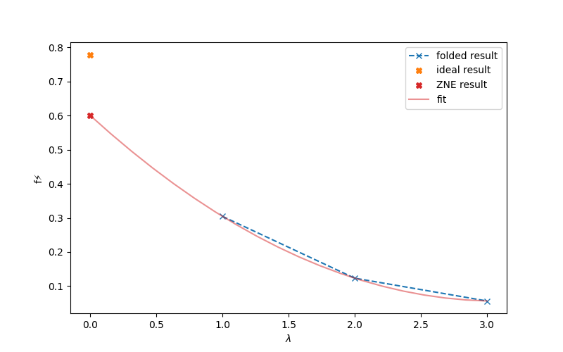
We see that the mitigated result comes close to the ideal result, whereas the noisy result is further off (see value at scale_factor=1).

Note that this folding scheme is relatively simple and only really is sensible for integer values of scale_factor. At the same time, scale_factor is limited from above by the noise as the noisy quantum function quickly decoheres under this folding. I.e., for \(\lambda\geq 4\) the results are typically already decohered. Therefore, one typically only uses scale_factors = [1, 2, 3]. In principle, one can think of more fine grained folding schemes and test them by providing custom folding operations. How this can be done in PennyLane with the given API is described in mitigate_with_zne().

Note that Richardson extrapolation, which we used to define the mitigated_qnode, is just a fancy way to describe a polynomial fit of order = len(x) - 1. Alternatively, you can use poly_extrapolate() and manually pass the order via a keyword argument extrapolate_kwargs={'order': 2}.

Differentiable mitigation in a variational quantum algorithm

We will now use mitigation while we optimize the parameters of our variational circuit to obtain the ground state of the Hamiltonian — this is the variational quantum eigensolving (VQE), see A brief overview of VQE. Then, we will compare VQE optimization runs for the ideal, noisy, and mitigated QNodes and see that the mitigated one comes close to the ideal (zero noise) results, whereas the noisy execution is further off.

def VQE_run(cost_fn, max_iter, stepsize=0.1):
    """VQE Optimization loop"""
    opt = qml.AdamOptimizer(stepsize=stepsize)

    # fixed initial guess
    w1 = np.ones((n_wires), requires_grad=True)
    w2 = np.ones((n_layers, n_wires - 1, 2), requires_grad=True)

    energy = []

    # Optimization loop
    for _ in range(max_iter):
        (w1, w2), prev_energy = opt.step_and_cost(cost_fn, w1, w2)

        energy.append(prev_energy)

    energy.append(cost_fn(w1, w2))

    return energy


max_iter = 70

energy_ideal = VQE_run(qnode_ideal, max_iter)
energy_noisy = VQE_run(qnode_noisy, max_iter)
energy_mitigated = VQE_run(qnode_mitigated, max_iter)

energy_exact = np.min(np.linalg.eigvalsh(qml.matrix(H)))

plt.figure(figsize=(8, 5))
plt.plot(energy_noisy, ".--", label="VQE E_noisy")
plt.plot(energy_mitigated, ".--", label="VQE E_mitigated")
plt.plot(energy_ideal, ".--", label="VQE E_ideal")
plt.plot([1, max_iter + 1], [energy_exact] * 2, "--", label="E_exact")
plt.legend(fontsize=14)
plt.xlabel("Iteration", fontsize=18)
plt.ylabel("Energy", fontsize=18)
plt.show()

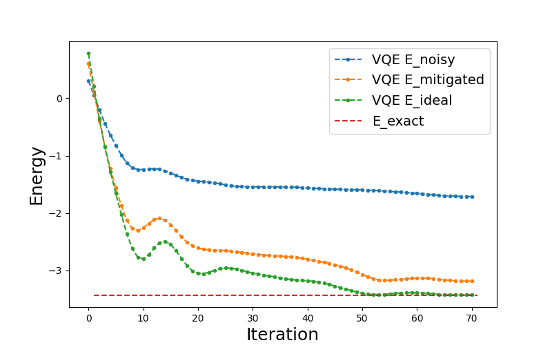
We see that during the optimization we are for the most part significantly closer to the ideal simulation and end up with a better energy compared to executing the noisy device without ZNE.

So far we have been using PennyLane gradient methods that use autograd for simulation and parameter-shift rules for real device executions. We can also use the other interfaces that are supported by PennyLane, jax, torch and tensorflow, in the usual way as described in the interfaces section of the documentation Gradients and training.

Differentiating the mitigation transform itself

In the previous sections, we have been concerned with differentiating through the mitigation transform. An interesting direction for future work is differentiating the transform itself 1. In particular, the authors in 2 make the interesting observation that for some error mitigation schemes, the cost function is smooth in some of the mitigation parameters. Here, we show one of their examples, which is a time-sensitive dynamical decoupling scheme:

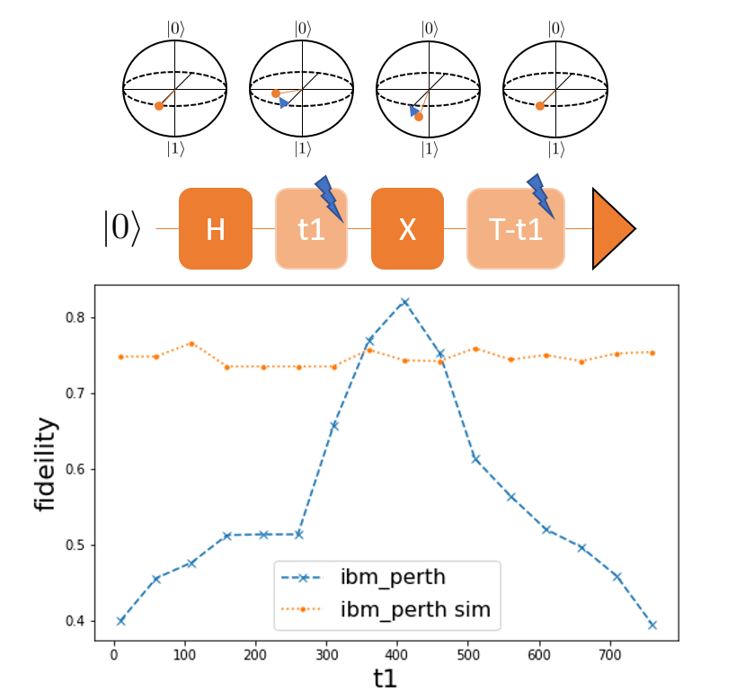
Time-sensitive dynamical decoupling scheme.

In this mitigation technique, the single qubit state is put into an equal superposition: \(|+\rangle = (|0\rangle + |1\rangle)/\sqrt{2}\). During the first idle time \(t_1\), the state is altered due to noise. Applying \(X\) reverses the roles of each computational basis state. The idea is that the noise in the second idle time \(T-t_1\) is cancelling out the effect of the first time window. We see that the output fidelity is a smooth function of \(t_1\). This was executed on ibm_perth, and we note that simple noise models, like the simulated IBM device, do not suffice to reproduce the behavior of the real device.

Obtaining the gradient with respect to this parameter is difficult. Formally, writing down the derivative of this transform with respect to the idle time in order to derive its parameter-shift rules would require access to the noise model. This is very difficult for a realistic scenario. Further, most mitigation parameters are integers and would have to be smoothed in a differentiable way. A simple but effective strategy is using finite differences for the gradient with respect to mitigation parameters.

Overall, this is a nice example of a mitigation scheme where varying the mitigation parameter has direct impact to the simulation result. It is therefore desirable to be able to optimize this parameter at the same time as we perform a variational quantum algorithm.

Conclusion

We demonstrated how zero-noise extrapolation can be seamlessly incorporated in a differentiable workflow in PennyLane to achieve better results. Further, the possibility of differentiating error mitigation transforms themselves has been discussed and we have seen that some mitigation schemes require execution on real devices or more advanced noise simulations.

References

1

Olivia Di Matteo, Josh Izaac, Tom Bromley, Anthony Hayes, Christina Lee, Maria Schuld, Antal Száva, Chase Roberts, Nathan Killoran. “Quantum computing with differentiable quantum transforms.” arXiv:2202.13414, 2021.

2

Gokul Subramanian Ravi, Kaitlin N. Smith, Pranav Gokhale, Andrea Mari, Nathan Earnest, Ali Javadi-Abhari, Frederic T. Chong. “VAQEM: A Variational Approach to Quantum Error Mitigation.” arXiv:2112.05821, 2021.

About the author

Korbinian Kottmann

Korbinian is a Quantum Scientist at Xanadu, interested in quantum simulation and quantum software.

demos/tutorial_diffable-mitigation

 

Download Python script

 

Download Notebook

 

View on GitHub