Note
Click here to download the full example code
Optimizing noisy circuits with Cirq
Author: Nathan Killoran — Posted: 01 June 2020. Last updated: 16 June 2021.
Until we have fault-tolerant quantum computers, we will have to learn to live with noise. There are lots of exciting ideas and algorithms in quantum computing and quantum machine learning, but how well do they survive the reality of today’s noisy devices?
Background
Quantum pure-state simulators are great and readily available in a number of quantum software packages. They allow us to experiment, prototype, test, and validate algorithms and research ideas—up to a certain number of qubits, at least.
But present-day hardware is not ideal. We’re forced to confront decoherence, bit flips, amplitude damping, and so on. Does the presence of noise in near-term devices impact their use in, for example, variational quantum algorithms? Won’t our models, trained so carefully in simulators, fall apart when we run on noisy devices?
In fact, there is some optimism that variational algorithms may be the best type of algorithms on near-term devices, and could have an in-built adaptability to noise that more rigid textbook algorithms do not possess. Variational algorithms are somewhat robust against the fact that the device they are run on may not be ideal. Being variational in nature, they can be tuned to “work around” noise to some extent.
Quantum machine learning leverages a lot of tools from its classical counterpart. Fortunately, there is great evidence that machine learning algorithms can not only be robust to noise, but can even benefit from it! Examples include the use of reduced-precision arithmetic in deep learning, the strong performance of stochastic gradient descent, and the use of “dropout” noise to prevent overfitting.
With this evidence to motivate us, we can still hope to find, extract, and work with the underlying quantum “signal” that is influenced by a device’s inherent noise.
Noisy circuits: creating a Bell state
Let’s consider a simple quantum circuit which performs a standard quantum information task: the creation of an entangled state and the measurement of a Bell inequality (also known as the CHSH inequality).
Since we’ll be dealing with noise, we’ll need to use a simulator that supports noise and density-state representations of quantum states (in contrast to many simulators, which use a pure-state representation).
Fortunately, Cirq provides mixed-state simulators and noisy operations natively, so we can use the PennyLane-Cirq plugin to carry out our noisy simulations.
import pennylane as qml
from pennylane import numpy as np
import matplotlib.pyplot as plt

dev = qml.device("cirq.mixedsimulator", wires=2, shots=1000)

# CHSH observables
A1 = qml.PauliZ(0)
A2 = qml.PauliX(0)
B1 = qml.Hermitian(np.array([[1, 1], [1, -1]]) / np.sqrt(2), wires=1)
B2 = qml.Hermitian(np.array([[1, -1], [-1, -1]]) / np.sqrt(2), wires=1)
CHSH_observables = [A1 @ B1, A1 @ B2, A2 @ B1, A2 @ B2]


# subcircuit for creating an entangled pair of qubits
def bell_pair():
    qml.Hadamard(wires=0)
    qml.CNOT(wires=[0, 1])


# circuits for measuring each distinct observable
@qml.qnode(dev)
def measure_A1B1():
    bell_pair()
    return qml.expval(A1 @ B1)


@qml.qnode(dev)
def measure_A1B2():
    bell_pair()
    return qml.expval(A1 @ B2)


@qml.qnode(dev)
def measure_A2B1():
    bell_pair()
    return qml.expval(A2 @ B1)


@qml.qnode(dev)
def measure_A2B2():
    bell_pair()
    return qml.expval(A2 @ B2)


# now we measure each circuit and construct the CHSH inequality
expvals = [measure_A1B1(), measure_A1B2(), measure_A2B1(), measure_A2B2()]

# The CHSH operator is A1 @ B1 + A1 @ B2 + A2 @ B1 - A2 @ B2
CHSH_expval = np.sum(expvals[:3]) - expvals[3]
print(CHSH_expval)
Out:
2.776
The output here is \(2\sqrt{2}\), which is the maximal value of the CHSH inequality. States which have a value \(\langle CHSH \rangle \geq 2\) can safely be considered “quantum”.
Note
In this situation “quantum” means that there is no local hidden variable theory which could produce these measurement outcomes. It does not strictly mean the presence of entanglement.
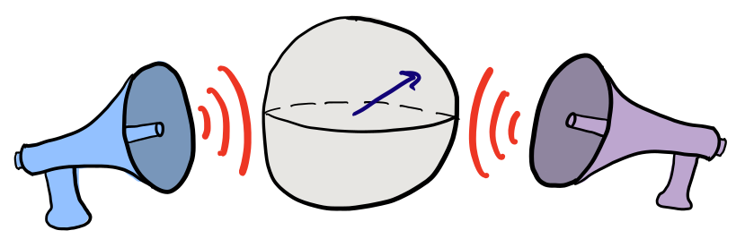
Now let’s turn up the noise! 📢 📢 📢
Cirq provides a number of noisy channels that are not part of PennyLane core. This is no issue, as the PennyLane-Cirq plugin provides these and allows them to be used directly in PennyLane circuit declarations.
from pennylane_cirq import ops as cirq_ops

# Note that the 'Operation' op is a generic base class
# from PennyLane core.
# All other ops are provided by Cirq.
available_ops = [op for op in dir(cirq_ops) if not op.startswith("_")]
print("\n".join(available_ops))
Out:
AmplitudeDamp
BitFlip
Depolarize
Operation
PhaseDamp
PhaseFlip
PennyLane operations and external framework-specific operations can be interwoven freely in circuits that use that plugin’s device for execution. In this case, the Cirq-provided channels can be used with Cirq’s mixed-state simulator.
We’ll use the BitFlip channel, which has the effect of
randomly flipping the qubits in the computational basis.
noise_vals = np.linspace(0, 1, 25)

CHSH_vals = []
noisy_expvals = []

for p in noise_vals:
    # we overwrite the bell_pair() subcircuit to add
    # extra noisy channels after the entangled state is created
    def bell_pair():
        qml.Hadamard(wires=0)
        qml.CNOT(wires=[0, 1])
        cirq_ops.BitFlip(p, wires=0)
        cirq_ops.BitFlip(p, wires=1)

    # measuring the circuits will now use the new noisy bell_pair() function
    expvals = [measure_A1B1(), measure_A1B2(), measure_A2B1(), measure_A2B2()]
    noisy_expvals.append(expvals)
noisy_expvals = np.array(noisy_expvals)
CHSH_expvals = np.sum(noisy_expvals[:, :3], axis=1) - noisy_expvals[:, 3]

# Plot the individual observables
plt.plot(noise_vals, noisy_expvals[:, 0], "D", label=r"$\hat{A1}\otimes \hat{B1}$", markersize=5)
plt.plot(noise_vals, noisy_expvals[:, 1], "x", label=r"$\hat{A1}\otimes \hat{B2}$", markersize=12)
plt.plot(noise_vals, noisy_expvals[:, 2], "+", label=r"$\hat{A2}\otimes \hat{B1}$", markersize=10)
plt.plot(noise_vals, noisy_expvals[:, 3], "v", label=r"$\hat{A2}\otimes \hat{B2}$", markersize=10)
plt.xlabel("Noise parameter")
plt.ylabel(r"Expectation value $\langle \hat{A}_i\otimes\hat{B}_j\rangle$")
plt.legend()
plt.show()
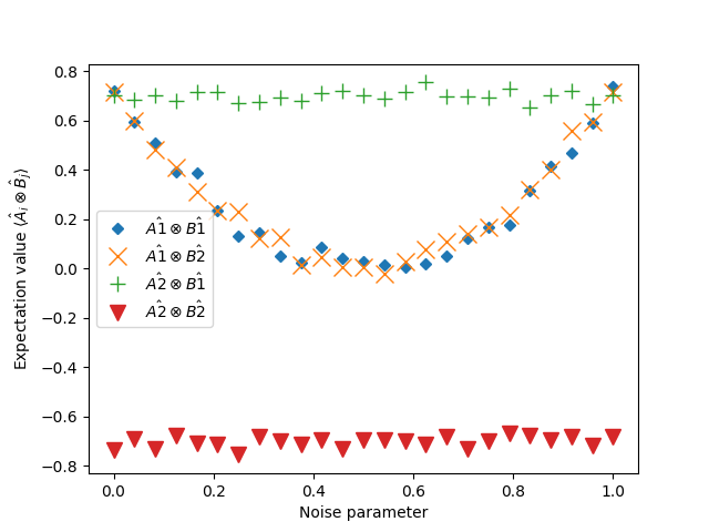
By adding the bit-flip noise, we have degraded the value of the CHSH observable. The first two observables \(\hat{A}_1\otimes \hat{B}_1\) and \(\hat{A}_1\otimes \hat{B}_2\) are sensitive to this noise parameter. Their value is weakened when the noise parameter is not 0 or 1 (note that the the CHSH operator is symmetric with respect to bit flips).
The latter two observables, on the other hand, are seemingly unaffected by the noise at all.
We can see that even when noise is present, there may still be subspaces or observables which are minimally affected or unaffected. This gives us some hope that variational algorithms can learn to find and exploit such noise-free substructures on otherwise noisy devices.
We can also plot the CHSH observable in the noisy case. Remember, values greater than 2 can safely be considered “quantum”.
plt.plot(noise_vals, CHSH_expvals, label="CHSH")
plt.plot(noise_vals, 2 * np.ones_like(noise_vals), label="Quantum-classical boundary")
plt.xlabel("Noise parameter")
plt.ylabel("CHSH Expectation value")
plt.legend()
plt.show()
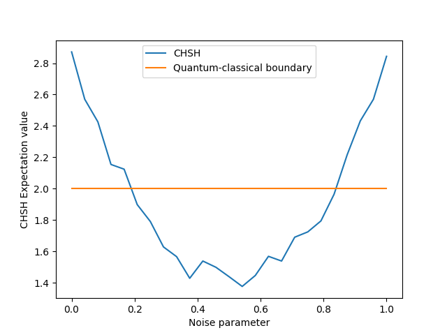
Too much noise (around 0.2 in this example), and we lose the quantumness we created in our circuit. But if we only have a little noise, the quantumness undeniably remains. So there is still hope that quantum algorithms can do something useful, even on noisy near-term devices, so long as the noise is not high.
Note
In Google’s quantum supremacy paper 1, they were able to show that some small signature of quantumness remained in their computations, even after a deep many-qubit noisy circuit was executed.
Optimizing noisy circuits
Now, how does noise affect the ability to optimize or train a variational circuit?
Let’s consider an analog of the basic qubit rotation tutorial, but where we add an extra noise channel after the gates.
Note
We model the noise process as the application of ideal noise-free gates, followed by the action of a noisy channel. This is a common technique for modelling noise, but may not be appropriate for all situations.
@qml.qnode(dev)
def circuit(gate_params, noise_param=0.0):
    qml.RX(gate_params[0], wires=0)
    qml.RY(gate_params[1], wires=0)
    cirq_ops.Depolarize(noise_param, wires=0)
    return qml.expval(qml.PauliZ(0))


gate_pars = [0.54, 0.12]
print("Expectation value:", circuit(gate_pars))
Out:
Expectation value: 0.864
In this case, the depolarizing channel degrades the qubit’s density matrix \(\rho\) towards the state
(at the value \(p=\frac{3}{4}\), it passes through the
maximally mixed state).
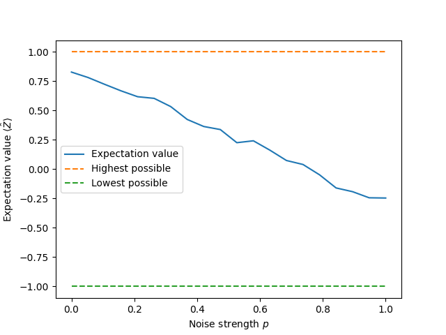
We can see this in our circuit by looking at how the final
PauliZ expectation value changes as
a function of the noise strength.
noise_vals = np.linspace(0.0, 1.0, 20)
expvals = [circuit(gate_pars, noise_param=p) for p in noise_vals]

plt.plot(noise_vals, expvals, label="Expectation value")
plt.plot(noise_vals, np.ones_like(noise_vals), "--", label="Highest possible")
plt.plot(noise_vals, -np.ones_like(noise_vals), "--", label="Lowest possible")
plt.ylabel(r"Expectation value $\langle \hat{Z} \rangle$")
plt.xlabel(r"Noise strength $p$")
plt.legend()
plt.show()
Let’s fix the noise parameter and see how the noise affects the
optimization of our circuit. The goal is the same as the
qubit rotation tutorial,
i.e., to tune the qubit state until it has a PauliZ expectation value
of \(-1\) (the lowest possible).
# declare the cost functions to be optimized
def cost(x):
    return circuit(x, noise_param=0.0)


def noisy_cost(x):
    return circuit(x, noise_param=0.3)


# initialize the optimizer
opt = qml.GradientDescentOptimizer(stepsize=0.4)

# set the number of steps
steps = 100
# set the initial parameter values
init_params = np.array([0.011, 0.055], requires_grad=True)
noisy_circuit_params = init_params
params = init_params

for i in range(steps):
    # update the circuit parameters
    # we can optimize both in the same training loop
    params = opt.step(cost, params)
    noisy_circuit_params = opt.step(noisy_cost, noisy_circuit_params)

    if (i + 1) % 5 == 0:
        print(
            "Step {:5d}. Cost: {: .7f}; Noisy Cost: {: .7f}".format(
                i + 1, cost(params), noisy_cost(noisy_circuit_params)
            )
        )

print("\nOptimized rotation angles (noise-free case):")
print("({: .7f}, {: .7f})".format(*params))
print("Optimized rotation angles (noisy case):")
print("({: .7f}, {: .7f})".format(*noisy_circuit_params))
Out:
Step     5. Cost:  0.9340000; Noisy Cost:  0.6080000
Step    10. Cost:  0.0180000; Noisy Cost:  0.5200000
Step    15. Cost: -0.9800000; Noisy Cost:  0.1980000
Step    20. Cost: -1.0000000; Noisy Cost: -0.4200000
Step    25. Cost: -1.0000000; Noisy Cost: -0.5780000
Step    30. Cost: -1.0000000; Noisy Cost: -0.6180000
Step    35. Cost: -1.0000000; Noisy Cost: -0.5800000
Step    40. Cost: -1.0000000; Noisy Cost: -0.6160000
Step    45. Cost: -1.0000000; Noisy Cost: -0.5600000
Step    50. Cost: -0.9960000; Noisy Cost: -0.5960000
Step    55. Cost: -1.0000000; Noisy Cost: -0.5840000
Step    60. Cost: -1.0000000; Noisy Cost: -0.6240000
Step    65. Cost: -1.0000000; Noisy Cost: -0.5720000
Step    70. Cost: -1.0000000; Noisy Cost: -0.6360000
Step    75. Cost: -1.0000000; Noisy Cost: -0.5840000
Step    80. Cost: -1.0000000; Noisy Cost: -0.6200000
Step    85. Cost: -0.9980000; Noisy Cost: -0.6020000
Step    90. Cost: -1.0000000; Noisy Cost: -0.5600000
Step    95. Cost: -1.0000000; Noisy Cost: -0.5820000
Step   100. Cost: -1.0000000; Noisy Cost: -0.5780000

Optimized rotation angles (noise-free case):
(-0.0010000,  3.1438000)
Optimized rotation angles (noisy case):
( 0.0170000,  3.1482000)
There are a couple interesting observations here:
The noisy circuit isn’t able to achieve the same final cost function value as the ideal circuit. This is because the noise causes the state to become irreversibly mixed. Mixed states can’t achieve the same extremal expectation values as pure states.
However, both circuits still converge to the same parameter values \((0,\pi)\), despite having different final states.
It could have been the case that noisy devices irreparably damage the optimization of variational circuits, steering us towards parameter values which are not at all useful. Luckily, at least for the simple example above, this is not the case. Optimizations on noisy devices can still lead to similar parameter values as when we run on ideal devices.
Understanding the effect of noisy channels
Let’s dig a bit into the underlying quantum information theory to understand better what’s happening 2. Expectation values of variational circuits, like the one we are measuring, are composed of three pieces:
an initial quantum state \(\rho\) (usually the zero state);
a parameterized unitary transformation \(U(\theta)\)); and
measurement of a final observable \(\hat{B}\).
The equation for the expectation value is given by the Born rule:
When optimizing, we can compute gradients of many common gates using the parameter-shift rule:
In our example, the parametrized unitary \(U(\theta)\) is split into two gates, \(U = U_2 U_1\), where \(U_1=R_X\) and \(U_1=R_Y\), and each takes an independent parameter \(\theta_i\).
What happens when we apply a noisy channel \(\Lambda\) after the gates? In this case, the expectation value is now taken with respect to the noisy circuit:
Thus, we can treat it as the expectation value of the same observable, but with respect to a different state \(\rho' = \Lambda\left[U(\theta)\rho U^\dagger(\theta)\right]\).
Alternatively, using the Heisenberg picture, we can transfer the channel \(\Lambda\) acting on the state \(U(\theta)\rho U^\dagger(\theta)\) into the adjoint channel \(\Lambda^\dagger\) acting on the observable \(\hat{B}\), transforming it to a new observable \(\hat{B} = \Lambda^\dagger[\hat{B}]=\hat{B}'\).
With the channel present, the expectation value can be interpreted as if we had the same variational state, but measured a different observable:
This has immediate consequences for the parameter-shift rule. With the channel present, we have simply
In other words, the parameter-shift rule continues to hold for all gates, even when we have additional noise!
Note
In the above derivation, we implicitly assumed that the channel does not depend on the variational circuit’s parameters. If the channel depended on the particular state, or if it depended on the parameters \(\theta\), we would need to be more careful.
Let’s confirm the above derivation with an example.
angles = np.linspace(0, 2 * np.pi, 50)
theta2 = np.pi / 4


def param_shift(theta1):
    return 0.5 * (
        noisy_cost([theta1 + np.pi / 2, theta2]) - noisy_cost([theta1 - np.pi / 2, theta2])
    )


noisy_expvals = [noisy_cost([theta1, theta2]) for theta1 in angles]
noisy_param_shift = [param_shift(theta1) for theta1 in angles]

plt.plot(angles, noisy_expvals, label="Expectation value")  # looks like 0.4 * cos(phi)
plt.plot(angles, noisy_param_shift, label="Parameter-shift value")  # looks like -0.4 * sin(phi)
plt.ylabel(r"Expectation value $\langle \hat{Z} \rangle$")
plt.xlabel(r"Angle $\theta_1$")
plt.legend()
plt.show()
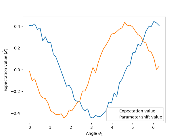
By inspecting the two curves, we can see that the parameter-shift rule gives the correct gradient of the expectation value, even with the presence of the noisy channel!
In this example, the influence of the channel is to attenuate the maximal amplitude that the qubit state can achieve (\(\approx 0.4\)). But even though the qubit’s amplitude is attenuated, the gradient computed by the parameter-shift rule still “points in the right direction”.
This backs up the observation we made earlier that the result of the optimization gave the correct values for the angle parameters, but the value of the final cost function was lower than the noise-free case.
Interpreting noisy circuit optimizations
Despite the observations that we can compute gradients for noisy channels, and that optimization may lead to the same parameter values for both noise-free and noisy circuits, we must still remain cautious in how we interpret the results.
We can evaluate the correct gradient for the expectation value
but, because the noisy channel is present, this expectation value may not reflect the actual expectation value we wanted to compute. This is important to keep in mind for certain algorithms that have a physical interpretation for the variational circuit.
For example, in the variational quantum eigensolver, we want to find the ground-state energy of a physical system. If there is an appreciable amount of noise present, the state we are optimizing will necessarily become mixed, and we should be careful interpreting the optimum value as the exact ground-state energy.
References
- 1
Frank Arute et al. “Quantum supremacy using a programmable superconducting processor.” Nature, 574(7779), 505-510.
- 2
Johannes Jakob Meyer, Johannes Borregaard, and Jens Eisert. “A variational toolbox for quantum multi-parameter estimation.” arXiv:2006.06303, 2020.